7 3D Laminar Flat-Plate Boundary Layer — PBNS Blasius Verification
Verification of the constant-density pressure-based solver against the Blasius velocity profile and skin-friction solution
7.1 Run Provenance and Artifacts
| Item | Value |
|---|---|
| Wake CFD baseline version | 0.22.2 |
| Solver | PBNS |
| Compute device | GPU (NVIDIA RTX A2000) |
| Parallel execution | 1 MPI rank |
| Arithmetic precision | FP64 |
| Run date | 2026-09-23 |
Results depend on the solver build that produced them. Read every figure in this report together with the version and date above — re-running the same input on a later build may give different numbers.
7.1.1 Downloadable Files
Not available: standalone input decks and solver result files have not yet been published for download.
7.2 Verification Objective
This case simulates a steady, constant-density laminar boundary layer over a flat plate with Wake CFD’s pressure-based Navier–Stokes (PBNS) solver. It compares the computed velocity profiles and local skin-friction coefficient with the Blasius similarity solution to verify:
- the incompressible, constant-density PBNS formulation for a low-speed external flow
- no-slip wall treatment and viscous momentum diffusion
- pressure–velocity coupling on a three-dimensional mesh
- recovery of the Blasius similarity profile and wall shear at
Re_L=1×10^5
The physical setup follows the DBNS laminar flat-plate case, while the two-dimensional mesh is extruded by one cell in the spanwise direction because PBNS uses the three-dimensional solver path. Only the incompressible result is reported here; no compressible low-Mach or heat-transfer result is included.
7.3 Reference Solution and Data
7.3.1 Analytical Solution
Let x denote distance from the plate leading edge, y the wall-normal distance, U_inf the inlet velocity, and nu=mu/rho the kinematic viscosity. The similarity coordinate and local Reynolds number are
\[ \eta = y\sqrt{\frac{U_\infty}{\nu x}}, \qquad Re_x = \frac{U_\infty x}{\nu}. \]
The Blasius solution gives u/U_inf=f'(eta) and
\[ C_f(x)=\frac{0.664}{\sqrt{Re_x}}, \qquad \delta_{99}\approx 4.91\sqrt{\frac{\nu x}{U_\infty}}. \]
Velocity profiles at different streamwise stations should therefore collapse onto one curve when plotted in similarity coordinates.
7.4 Simulation Conditions
| Item | Setting |
|---|---|
| Dimension | 3D, one-cell spanwise extrusion |
| Domain | x=[0, 0.762] m, y=[0, 0.1524] m, z=[0, 0.003048] m |
| Flat plate | x=[0.1524, 0.4572] m, L=0.3048 m |
| Analysis | Steady, laminar PBNS, incompressible constant-density Navier–Stokes |
| Density | rho=1.1827 kg/m^3 |
| Dynamic viscosity | mu=1.8×10^-5 Pa·s |
| Inlet velocity | U_inf=4.994 m/s |
| Reynolds number | Re_L≈1.0×10^5 |
| Reference pressure | 101325 Pa |
7.5 Mesh
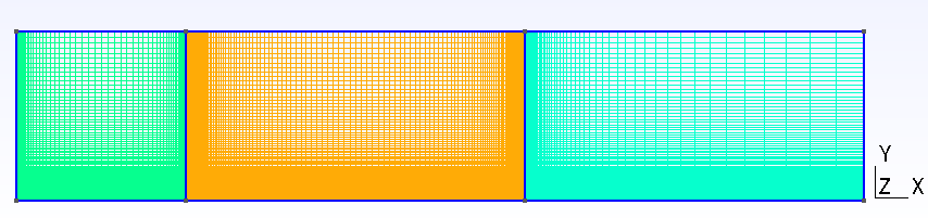
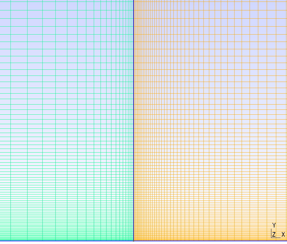
The mesh contains 58,050 nodes and 28,672 hexahedral cells. It is a one-cell spanwise extrusion of the same two-dimensional flat-plate mesh used by the DBNS case. The figures below show that shared two-dimensional plane; the PBNS mesh adds only the spanwise extrusion, with symmetry conditions on both extrusion faces.
7.6 Boundary and Initial Conditions
| Boundary | Type | Setting |
|---|---|---|
| Plate | Wall | no-slip |
| Bottom, upstream and downstream of plate | Symmetry | slip |
| Inlet | Velocity inlet | U=4.994 m/s in the streamwise direction |
| Outlet | Pressure outlet | p=101325 Pa |
| Top | Symmetry | slip |
| Front and back extrusion faces | Symmetry | one-cell spanwise slab |
Initial field: Not reported.
7.7 Numerical Methods
| Item | Setting |
|---|---|
| Solver | Coupled PBNS, constant density |
| Spatial discretization | Second order, Green–Gauss gradients |
| Pressure–velocity coupling | Rhie–Chow interpolation |
| Pseudo-time control | Constant convective CFL=1 |
| Linear solver | FGMRES, maximum 100 iterations, relative tolerance 10^-3 |
| Preconditioner | DILU, 5 sweeps |
| Outer-iteration limit | 2,000 |
| Configured convergence target | Scaled residual reduction of 10 orders |
The run reached the 2,000-iteration limit rather than the configured 10-order residual target. The combined flow scaled residual nevertheless decreased from 10^-3.41 at the first reported iteration to 10^-6.78 at the final iteration. The verification metrics below are evaluated from that final solution and are reported separately from the residual stopping condition.
7.8 Results
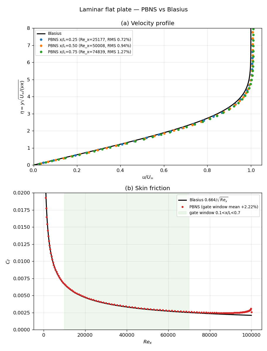
The velocity profile was sampled at three stations. RMS error was computed after interpolating each profile onto the Blasius reference points in similarity coordinates.
x/L |
Re_x |
RMS error in u/U_inf |
Computed delta_99 in similarity coordinates |
|---|---|---|---|
| 0.25 | 25,177 | 0.72% | 4.59 |
| 0.50 | 50,008 | 0.94% | 4.52 |
| 0.75 | 74,839 | 1.27% | 4.44 |
All three profiles remain within 1.3% RMS of the Blasius solution. The computed boundary-layer thickness is slightly below the Blasius value of approximately eta_99=4.91, with the difference increasing toward the trailing edge.
Local skin friction was reconstructed from the final solution using a second-order one-sided wall-normal velocity gradient. Over the assessment window 0.1<x/L<0.7, the mean relative difference from the Blasius relation is +2.224%. The window excludes the leading-edge singularity and the downstream portion where the finite plate and following slip boundary produce an increasing trailing-edge effect. Across the wider 0.1<x/L<0.9 interval, the mean absolute difference is 3.586% and the largest local difference is 10.349% near the end of that interval.
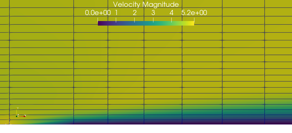
The velocity-magnitude field shows the expected boundary layer growing from the plate leading edge. Mesh lines are overlaid to show the wall-normal clustering used to resolve the near-wall gradient.
7.9 Conclusions and Applicable Scope
- The incompressible PBNS solution reproduces the Blasius velocity profile with
0.72–1.27%RMS error at the three sampled stations. - Mean local skin friction is
2.224%above the Blasius relation over the primary0.1<x/L<0.7assessment window. - The case confirms the constant-density PBNS pressure–velocity coupling, viscous wall treatment, and one-cell three-dimensional path for this steady laminar flow.
- The run stopped at its 2,000-iteration limit, at a final combined scaled residual of approximately
10^-6.78, rather than satisfying the configured 10-order target. - These results apply to one mesh and one Reynolds number for a zero-pressure-gradient, incompressible laminar boundary layer. They do not establish PBNS accuracy for turbulent flow, pressure gradients, separation, unsteady flow, or other Reynolds numbers.
This case fills the PBNS track in Wake CFD’s flat-plate verification family. The related DBNS and FR reports use the same physical baseline with solver-specific meshes and numerical methods.
7.10 References
- Blasius, H., “Grenzschichten in Flüssigkeiten mit kleiner Reibung,” Zeitschrift für Mathematik und Physik, 56, 1908, pp. 1–37.
- White, F.M., Viscous Fluid Flow, 3rd ed., McGraw-Hill, 2006 (Blasius similarity solution, Chapter 4).