14 2D Coflowing Jet — NASA TMR SA Verification
Code-to-code verification of thin-plate drag and free-shear-layer development against CFL3D and FUN3D, five-level grid convergence
14.1 Run Provenance and Artifacts
| Item | Value |
|---|---|
| Wake CFD baseline version | 0.22.2 |
| Solver | DBNS |
| Compute device | GPU (NVIDIA RTX A6000) |
| Parallel execution | 1 MPI rank |
| Arithmetic precision | FP64 |
| Run date | 2026-09-15 |
Results depend on the solver build that produced them. Read every figure in this report together with the version and date above — re-running the same input on a later build may give different numbers.
14.1.1 Downloadable Files
Not available: standalone input decks and solver result files have not yet been published for download.
14.2 Verification Objective
This case simulates a compressible free jet (M≈0.5) discharging alongside a coflow stream (M≈0.25) from a zero-thickness splitter plate, using the Spalart–Allmaras (SA) model. It compares Wake CFD against the NASA Turbulence Modeling Resource (TMR) 2D Coflowing Jet verification case, which is explicitly designed by TMR as a code-to-code verification case (not an experiment-matching case) and provides CFL3D and FUN3D reference solutions on the same five-level grid family. It verifies Wake CFD for:
- thin-plate drag coefficient (
Cd) prediction and its grid-convergence trajectory - downstream centerline-velocity development in the merged free-shear layer
- eddy-viscosity distribution in the shear layer
- behavior of pressure-inflow boundary conditions for two adjacent streams at different total pressure and temperature
14.3 Reference Solution and Data
The TMR coflowing-jet case places a zero-thickness splitter plate (adiabatic, no-slip on both sides) between an inner jet stream and an outer coflow stream. Downstream of the plate trailing edge, the two streams merge into a free-shear layer. The reference solutions (CFL3D, cell-centered; FUN3D, node-centered) are computed on the same mesh family, both using the Roe scheme, which makes the comparison a genuine code-to-code discretization check rather than a physical-model comparison. Reference values are taken directly from TMR’s published convergence.dat and profile data files.
| Item | Setting |
|---|---|
| References | CFL3D and FUN3D, both SA + Roe FDS on the same mesh, published by NASA TMR |
14.4 Simulation Conditions
| Item | Setting |
|---|---|
| Geometry | Splitter plate at −10 < x < 0, y = 0.5 (zero thickness); domain −10 < x < 200, 0 < y < 100 |
| Analysis | Steady, compressible DBNS, RANS (Spalart–Allmaras) |
| Inner jet stream | Pt/p∞ = 1.1862, Tt/T∞ = 1.050 (M ≈ 0.5) |
| Outer coflow stream | Pt/p∞ = 1.046, Tt/T∞ = 1.000 (M ≈ 0.25) |
14.5 Mesh
| Item | Setting |
|---|---|
| Mesh | Unstructured quadrilateral, single-cell spanwise extrusion; five-level nested grid family, 1,280–327,680 cells |
14.6 Boundary and Initial Conditions
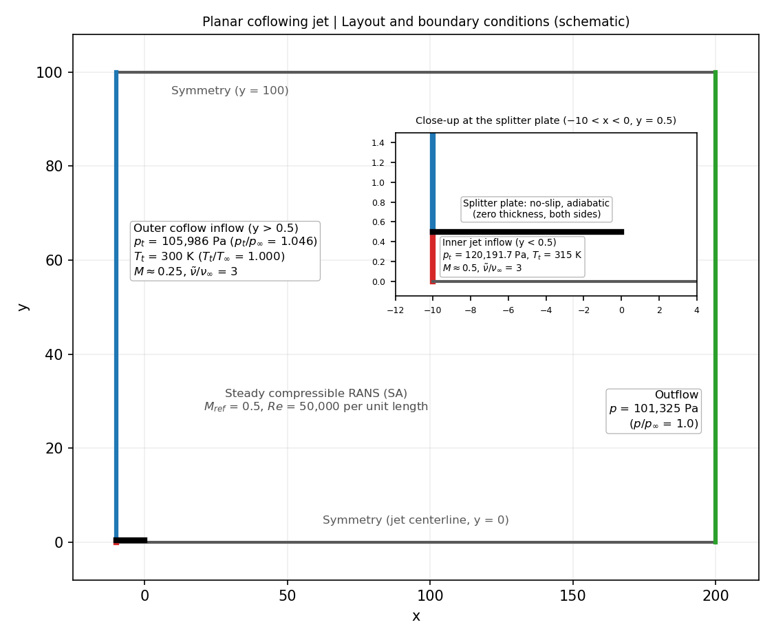
The schematic was drawn from the simulation inputs and the geometry published by NASA TMR (inflow at x = -10, outflow at x = 200, splitter plate at y = 0.5).
| Boundary | Condition |
|---|---|
Inner jet inflow (y < 0.5) |
Total-pressure inlet, p_t = 120,191.7 Pa (p_t/p∞ = 1.1862), T_t = 315 K (T_t/T∞ = 1.050), flow direction +x |
Outer coflow inflow (y > 0.5) |
Total-pressure inlet, p_t = 105,986 Pa (p_t/p∞ = 1.046), T_t = 300 K (T_t/T∞ = 1.000), flow direction +x |
Outflow (x = 200) |
Pressure outlet, back pressure 101,325 Pa (p/p∞ = 1.0) |
Jet centerline (y = 0) |
Symmetry |
Upper boundary (y = 100) |
Symmetry (not a farfield condition) |
| Splitter plate, both sides | No-slip, adiabatic wall |
| Spanwise faces | Symmetry (the mesh is a one-cell extrusion) |
The reference state is p∞ = 101,325 Pa and T∞ = 300 K (540 °R in the TMR specification), M_ref = 0.5, and Re = 50,000 per unit grid length. The turbulence working variable at both inflows is ν̃/ν∞ = 3. The initial field is uniform, with M = 0.5, p = 101,325 Pa, T = 300 K, and flow direction +x.
14.7 Numerical Methods
| Item | Setting |
|---|---|
| Convective scheme | Roe, UMUSCL (κ=0.5), no limiter |
| Gradient method | Green–Gauss |
| Time integration | Euler implicit |
| CFL | Constant, 50 |
| Convergence criterion | Absolute residual ≤ -12 (log10 RMS of the flow-equation residual) |
14.8 Results
14.8.1 Grid Convergence
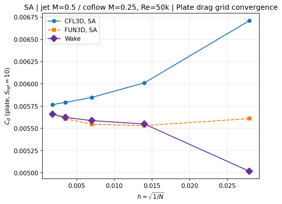
Reference profile and contour data are published only for the finest grid level; grid-convergence trajectories are compared across all five levels using TMR’s published convergence table.
| Grid level | Cells | Cd (Wake CFD) |
Cd (CFL3D) |
Cd (FUN3D) |
Wake CFD vs. FUN3D |
|---|---|---|---|---|---|
| 4 (coarsest) | 1,280 | 5.0172e-3 | 6.7104e-3 | 5.6094e-3 | −10.6% |
| 3 | 5,120 | 5.5485e-3 | 6.0111e-3 | 5.5304e-3 | +0.33% |
| 2 | 20,480 | 5.5865e-3 | 5.8473e-3 | 5.5453e-3 | +0.74% |
| 1 | 81,920 | 5.6228e-3 | 5.7914e-3 | 5.6075e-3 | +0.27% |
| 0 (finest) | 327,680 | 5.6603e-3 | 5.7658e-3 | 5.6648e-3 | −0.08% |
The finest-grid drag coefficient is within 0.08% of FUN3D and 1.8% of CFL3D. The two reference codes themselves differ from each other by up to 16% at the coarsest level and converge toward each other only on the two or three finest grids — the coarsest-level Wake CFD result (−10.6% vs. FUN3D) reflects the same discretization sensitivity, not a Wake CFD-specific error, since both reference codes also show large deviations from their own fine-grid values at that resolution. The plate-drag coefficient is a known difficult convergence metric for this case: TMR’s published observed order of convergence is p=1.13 for CFL3D and p=0.12 for FUN3D (the finest three levels remain outside the asymptotic range for FUN3D). Wake CFD’s convergence trajectory shows the same non-monotonic behavior as the FUN3D curve.
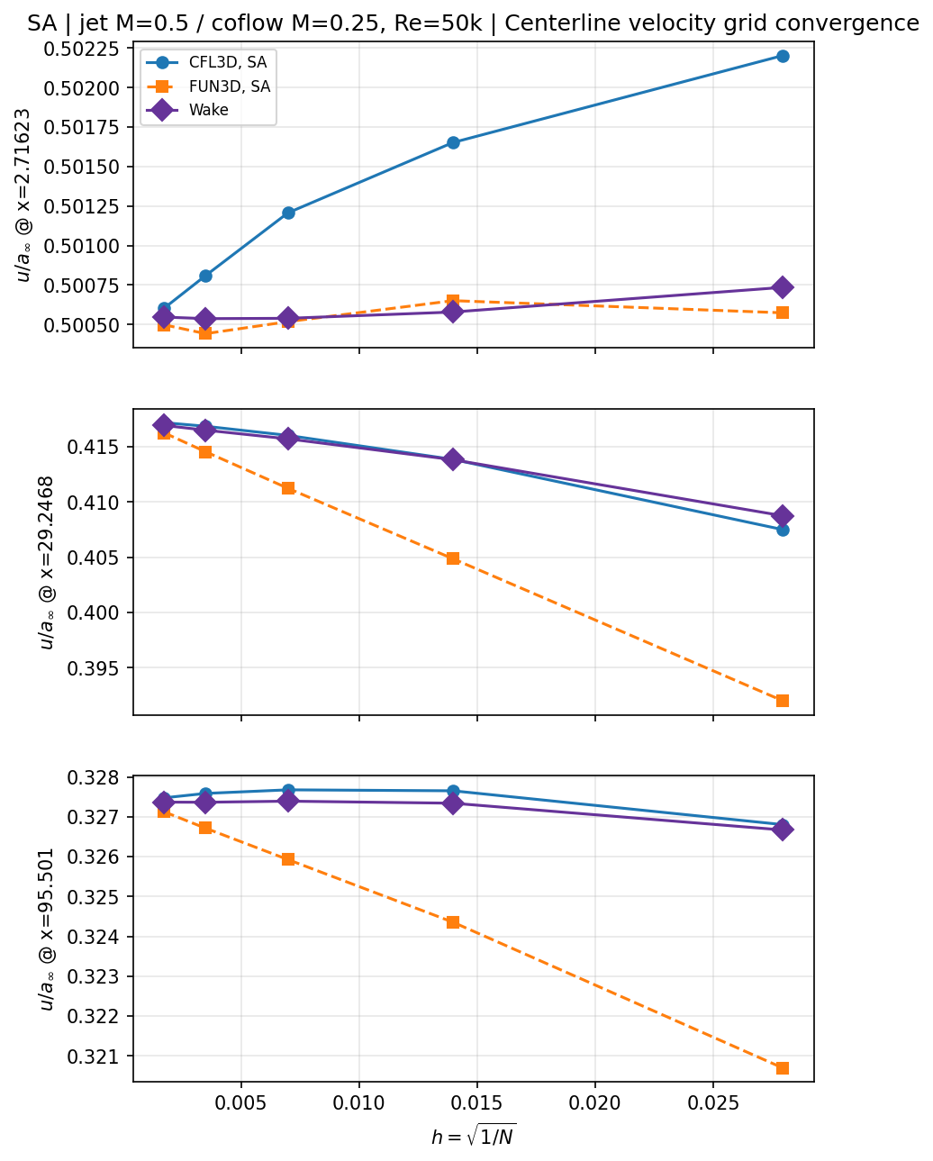
Centerline velocity at the three downstream stations (finest grid):
| Station | Wake CFD | CFL3D | FUN3D |
|---|---|---|---|
x = 2.71623 |
0.50055 | 0.50060 | 0.50049 |
x = 29.2468 |
0.41692 | 0.41717 | 0.41625 |
x = 95.501 |
0.32737 | 0.32748 | 0.32712 |
All three stations agree with both reference codes within the CFL3D–FUN3D band at every grid level.
14.8.2 Detailed Comparison on the Finest Grid
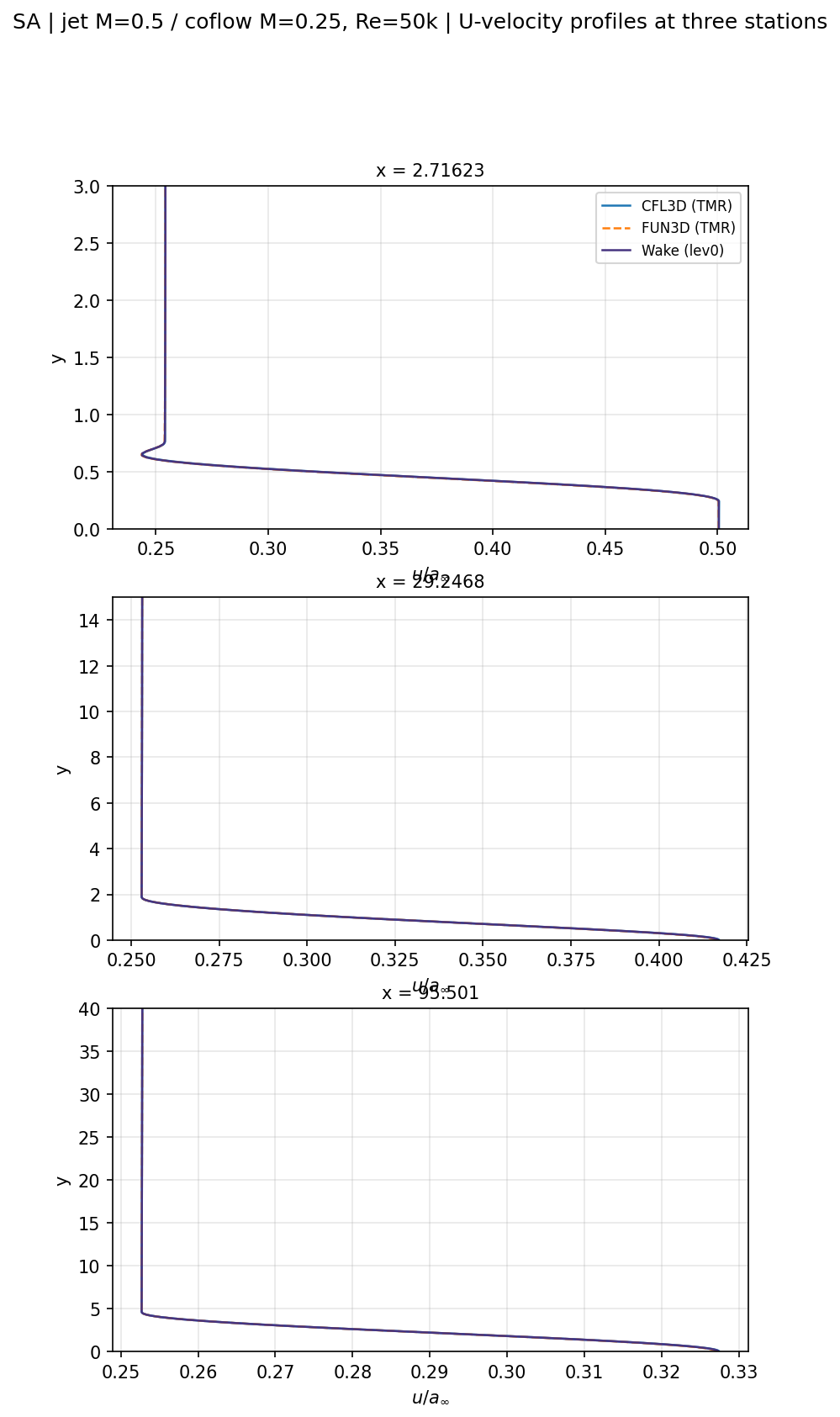
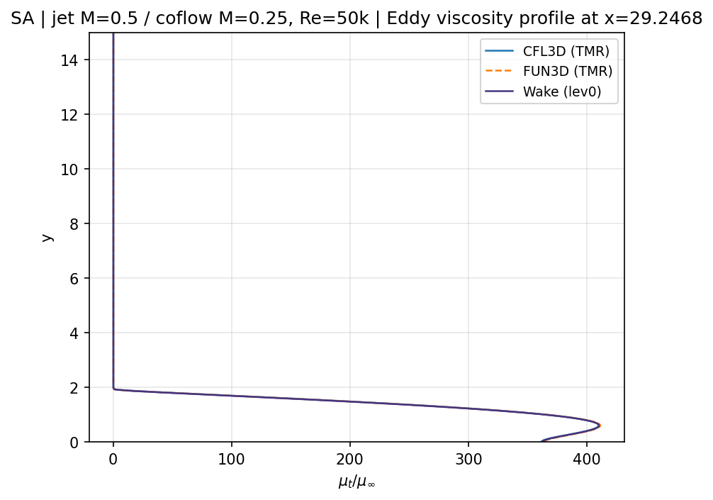
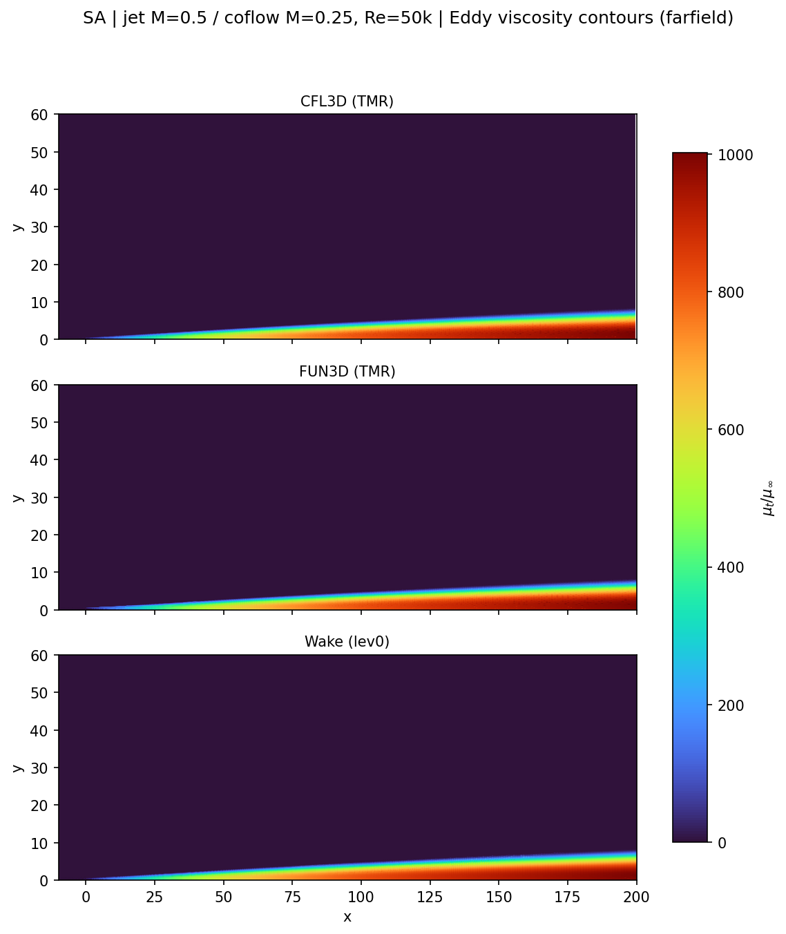
On the finest grid, Wake CFD’s velocity profiles, eddy-viscosity profile, and eddy-viscosity contours are visually indistinguishable from both reference codes.
14.9 Conclusions and Applicable Scope
- Wake CFD’s SA implementation agrees with the CFL3D and FUN3D reference solutions within the same code-to-code spread the two reference codes show against each other, for the full five-level grid family.
- On the finest grid, the plate-drag coefficient is within 0.08% of FUN3D and within 1.8% of CFL3D; all velocity and eddy-viscosity comparisons fall within the CFL3D–FUN3D band.
- This is a verification result: the reference is computed solutions from independent codes on the same mesh, not an experimental measurement. It establishes that Wake CFD solves the same discretized equations correctly for this compressible free-shear-layer and thin-plate-drag configuration.
- The result applies to a two-dimensional, compressible (
M≈0.5/M≈0.25), zero-thickness-plate free-shear-layer configuration at one Reynolds number. It does not establish accuracy against experimental turbulent free-shear-layer data (see the companion validation case for the planar mixing layer), three-dimensional effects, or other Mach-number combinations.
14.10 References
- NASA Turbulence Modeling Resource, 2D Coflowing Jet Verification Case and SA Expected Results.
- Bradbury, L. J. S., and Riley, J., “The Spread of a Turbulent Plane Jet Issuing into a Parallel Moving Airstream,” Journal of Fluid Mechanics, 27(2), 1967, pp. 381–394.