12 Conjugate Heat Transfer — Flat Plate Verification
Interface temperature and Nusselt number against the Vynnycky (1998) closed-form conjugate solution, 2D/3D and conformal/non-conformal interfaces
12.1 Run Provenance and Artifacts
| Item | Value |
|---|---|
| Wake CFD baseline version | 0.22.0 |
| Solver | DBNS |
| Compute device | GPU (NVIDIA RTX A6000) |
| Parallel execution | 1 MPI rank |
| Arithmetic precision | FP64 |
| Run date | 2026-08-29 |
Results depend on the solver build that produced them. Read every figure in this report together with the version and date above — re-running the same input on a later build may give different numbers.
12.1.1 Downloadable Files
Not available: standalone input decks and solver result files have not yet been published for download.
12.2 Verification Objective
This case checks Wake CFD’s conjugate heat transfer (CHT) capability — coupled fluid-solid heat conduction with continuity of temperature and heat flux at the interface — against the closed-form asymptotic solution of Vynnycky, Kimura, Kanev, and Pop (1998) for forced convection over a conducting flat plate. It verifies Wake CFD for:
- interface-averaged temperature (
θ̄_b) and Nusselt number (N̄u) against the analytical correlation - consistency between four independent discretization paths (2D/3D geometry, conformal/non-conformal fluid-solid interface mesh)
12.3 Reference Solution and Data
| Item | Setting |
|---|---|
| Reference | Vynnycky, Kimura, Kanev, and Pop (1998), closed-form asymptotic solution |
12.4 Simulation Conditions
| Item | Setting |
|---|---|
| Geometry | Conducting solid slab (x∈[-0.5,0.5], y∈[-0.5,0]) beneath a fluid domain (x∈[-1.0,2.0], y∈[0,1.0]); interface at y=0, |x|≤0.5 |
| Analysis | Steady, laminar, compressible DBNS with conjugate fluid-solid coupling |
Re (plate-length based) |
500 |
Pr |
0.72 |
Conductivity ratio k̄ = k_solid/k_fluid |
5 |
Thickness ratio λ = a/b |
0.5 |
| Freestream | M = 0.1, T_∞ = 300 K |
12.5 Mesh
| Item | Setting |
|---|---|
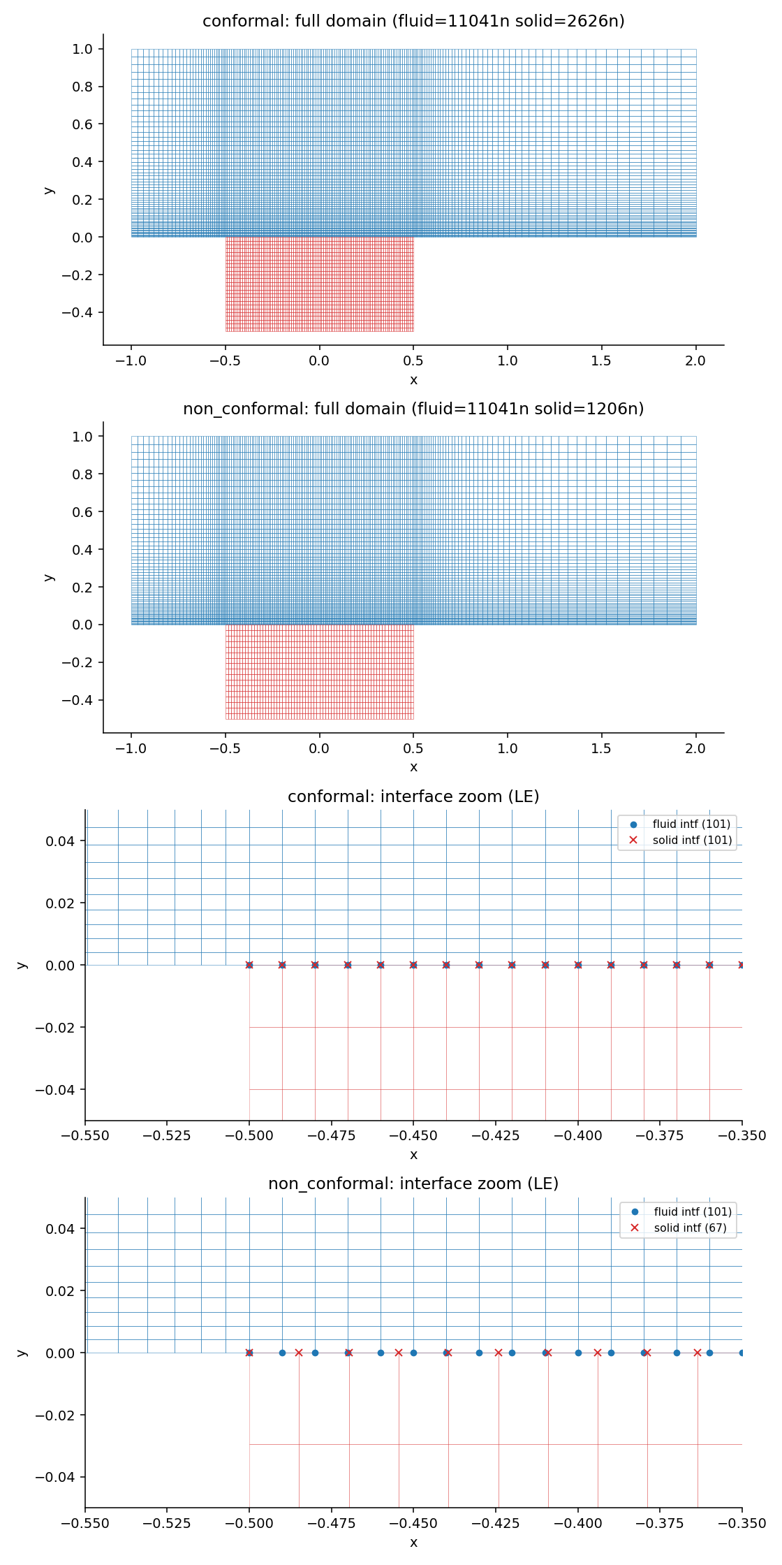
| Mesh variants | 2D and 3D (one-cell spanwise extrusion + symmetry), each with a conformal (matching interface node count) and non-conformal (mismatched, GGI-interpolated) fluid-solid interface |
12.6 Boundary and Initial Conditions
| Item | Setting |
|---|---|
| Solid bottom face | Isothermal, T_c = 330 K |
| Solid side faces | Adiabatic |
| Interface coupling | Temperature continuity (θ_solid = θ_fluid) and heat-flux continuity (∂θ_fluid/∂y = k̄·∂θ_solid/∂y) |
Initial field: Not reported.
12.7 Numerical Methods
| Item | Setting |
|---|---|
| Convective scheme | SLAU |
| Time integration | Implicit, CFL constant 5.0 |
| Convergence criterion | residual_reduction = 8 orders (deep convergence; confirmed against a 5,000-iteration snapshot with no meaningful difference) |
12.8 Results
At the given conditions (Re=500, Pr=0.72, k̄=5, λ=0.5), the analytical solution gives μ = λ·Pr^(1/3)·Re^(1/2) / (1.506·k̄) ≈ 1.331, θ̄_b = 1/(1+μ) ≈ 0.429, and N̄u = (k̄/λ)·μ/(1+μ) ≈ 5.71.
| Case | Converged iteration | θ̄_b (area-weighted) |
vs. analytical (0.429) |
N̄u |
vs. analytical (5.71) |
|---|---|---|---|---|---|
| 2D conformal | 10,637 | 0.4223 | −1.6% | 5.7738 | +1.1% |
| 2D non-conformal | 9,408 | 0.4251 | −0.9% | 5.8122 | +1.8% |
| 3D conformal | 13,023 | 0.4223 | −1.6% | 5.7738 | +1.1% |
| 3D non-conformal (GGI) | 11,873 | 0.4251 | −0.9% | 5.8122 | +1.8% |
All four discretization paths agree with the analytical correlation within 2%, inside the correlation’s own stated approximation error. The 2D and 3D results match to four decimal places (expected, since the 3D case is a one-cell spanwise extrusion of the same physical problem), which also confirms that the GGI interpolation used at the non-conformal interface does not degrade accuracy relative to the conformal case (difference between conformal and non-conformal results is about 0.3 percentage points).
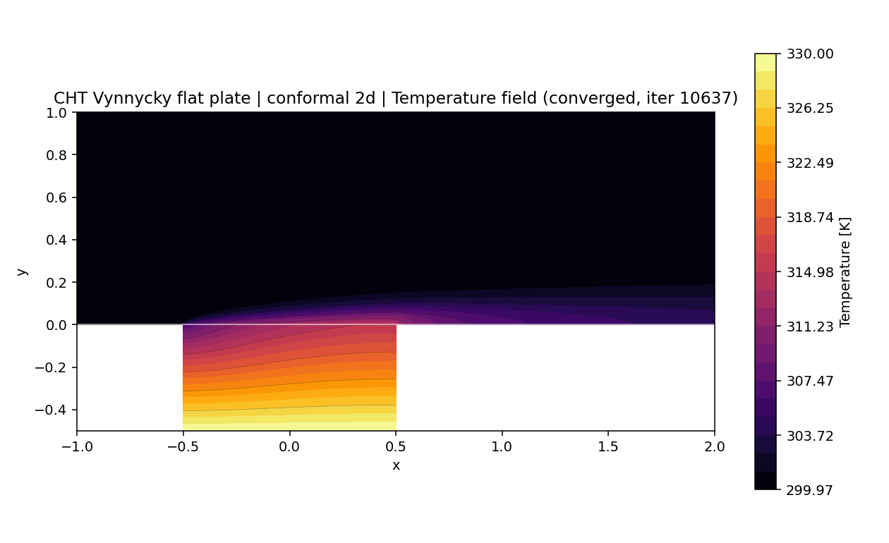
The local (as opposed to area-averaged) interface temperature distribution θ_b(x) was also compared against a separate constant-heat-flux asymptotic approximation from the same reference (valid, per the reference’s own statement, only for Pr≫1):
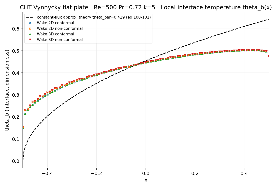
θ_b(x): Wake CFD (all four discretizations) versus the constant-flux approximation evaluated at Pr=0.72The area-averaged quantities (θ̄_b, N̄u) match well, but the local shape of θ_b(x) differs clearly from the constant-flux approximation. This is expected: that specific local approximation is derived and validated by its authors only for Pr≫1, and this case runs at Pr=0.72 — outside its stated range of applicability. It is not evidence against the CHT implementation; it is a direct measurement of that particular approximation’s scope of validity at a Pr value the original reference does not cover, as distinct from the general-Pr area-averaged correlation used above.
12.9 Conclusions and Applicable Scope
- Wake CFD’s conjugate heat transfer implementation reproduces the Vynnycky (1998) area-averaged interface temperature and Nusselt number within 2% across four independent discretization paths (2D/3D, conformal/non-conformal interface).
- The non-conformal (GGI-interpolated) interface path introduces no measurable accuracy penalty relative to the conformal path for this case.
- This result applies to steady, laminar, incompressible-regime forced convection over a flat conducting slab at one Reynolds number, Prandtl number, and conductivity/thickness ratio. It does not establish CHT accuracy for turbulent flow, unsteady conjugate problems, or other property ratios.
- The local interface temperature distribution does not match a
Pr≫1-specific asymptotic approximation at this case’sPr=0.72— consistent with that approximation’s own stated range of validity, not a discrepancy in the area-averaged result.
12.10 References
- Vynnycky, M., Kimura, S., Kanev, K., and Pop, I., “Forced Convection Heat Transfer from a Flat Plate: The Conjugate Problem,” International Journal of Heat and Mass Transfer, 41(1), 1998, pp. 45–59.