22 3D Transonic Wing — ONERA M6 RANS Validation
Wall-function spanwise pressure-coefficient validation against NASA WIND-US and the ONERA S2MA experiment
22.1 Run Provenance and Artifacts
| Item | Value |
|---|---|
| Wake CFD baseline version | 0.22.2 |
| Solver | DBNS |
| Compute device | GPU (NVIDIA RTX A6000) |
| Parallel execution | 1 MPI rank |
| Arithmetic precision | FP64 |
| Run date | 2026-09-22 |
Results depend on the solver build that produced them. Read every figure in this report together with the version and date above — re-running the same input on a later build may give different numbers.
22.1.1 Downloadable Files
Not available: standalone input decks and solver result files have not yet been published for download.
22.2 Validation Objective
The ONERA M6 half-wing is a classic transonic shock/boundary-layer-interaction case: a swept, tapered wing at moderate lift produces the characteristic “lambda” shock pattern on its upper surface, where two shock legs merge as they move outboard. This case compares Wake CFD’s spanwise surface-pressure distribution with both the original ONERA S2MA wind-tunnel experiment and NASA’s own WIND-US CFD solution for the same geometry and conditions, across a sweep of four convective schemes.
This case also validates Wake CFD’s wall-function near-wall treatment on a 3D swept wing. The mesh does not resolve the viscous sublayer (y+≈1); instead, the wall function reconstructs the near-wall velocity profile from a coarser first cell sized for y+≈30. This is the same near-wall treatment NASA specifies in its own reference WIND-US input (“wall function on”), so the comparison is apples-to-apples on wall treatment as well as on geometry and conditions — not an added source of discrepancy.
For users, this result supports review of 3D transonic wing pressure distributions and shock location during early design using a wall-function mesh, without needing to resolve the boundary layer with a y+≈1 mesh.
22.3 Reference Solution and Data
| Item | Setting |
|---|---|
| Reference | NASA GRC WIND-US ONERA M6 Wing validation archive (Study #1, m6wing01); original experiment: Schmitt & Charpin, AGARD AR-138 |
22.4 Simulation Conditions
| Item | Setting |
|---|---|
| Geometry | NASA GRC ONERA M6 half wing |
| Analysis | Steady, compressible RANS |
| Freestream Mach | 0.8395 |
| Angle of attack | 3.06° |
| Reynolds number | Re_MAC=11.72×10^6 (mean aerodynamic chord, MAC=0.540057 ft) |
22.5 Mesh
| Item | Setting |
|---|---|
| Mesh | Unstructured hexahedral, 294,912 cells / 306,577 points; first-cell spacing sized for the wall-function target, not boundary-layer-resolved |
22.6 Boundary and Initial Conditions
| Item | Setting |
|---|---|
| Wall treatment | Wall function (wall_function: standard) on the wing surface, target y+≈30 — matches the near-wall treatment in NASA’s own WIND-US reference input |
Why a wall function here. A y+≈1 wall-resolved mesh needs many more near-wall layers than a wall-function mesh at the same accuracy target, which increases cell count and run time substantially on a 3D wing. Using the wall function keeps this mesh at 294,912 cells while still reproducing the shock location and spanwise pressure distribution shown below.
Initial field: Not reported.
22.7 Numerical Methods
| Item | Setting |
|---|---|
| Turbulence model | Spalart–Allmaras (SA) |
| Convective schemes | Roe, HLLC, AUSM+up2, and SLAU2 (compared below) |
| Gradients / limiter | Green-Gauss physical gradient, unweighted least-squares reconstruction gradient, Venkatakrishnan limiter (coeff=0.01) |
| Time integration | Implicit, adaptive CFL (start 5, min 1, max 100) |
22.8 Results
22.8.1 Key Results
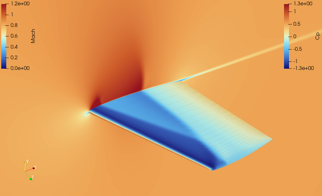
Cp and farfield Mach contour, showing the ONERA M6’s characteristic lambda-shock pattern where the shock’s two legs merge outboard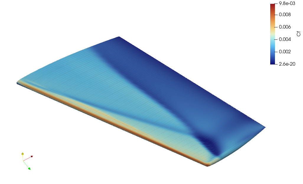
Cf drops locally follows the shock-foot line visible in the Cp/Mach contour above.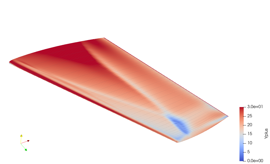
y+. Mostly 25-30 as targeted by the wall function, with a local dip at the shock foot.The y+ contour confirms the wall function is operating at its intended target across nearly the entire wing, dipping only locally where the shock impinges on the boundary layer.
22.8.2 Comparison with Experiment and NASA WIND-US
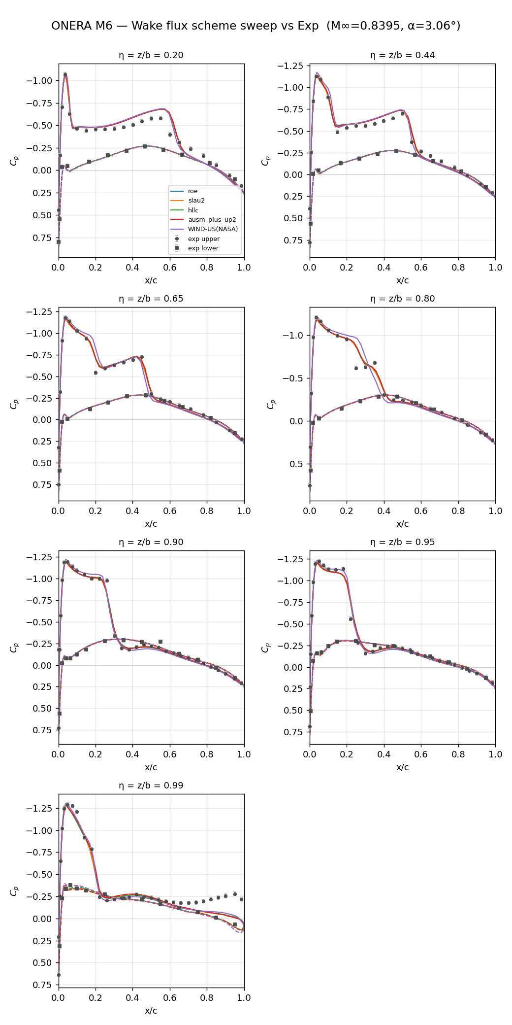
Across all seven spanwise stations (η=0.20 to 0.99), the four recommended schemes are essentially indistinguishable from each other and track both the WIND-US CFD solution and the experimental points closely, including the suction-side shock location and the leading-edge suction peak. The only visible departure is at η=0.80, where WIND-US places the shock slightly further upstream than either Wake CFD or the experiment.
22.8.3 Comparisons for Scheme Selection
All four schemes below converge normally with consistent lift and pressure distribution on this mesh and settings — the same four shown in the Cp comparison above.
| Scheme | CL |
CD |
Residual | Assessment |
|---|---|---|---|---|
| Roe | 0.2664 | 0.0190 | 7.21 | Default choice |
| HLLC | 0.2675 | 0.0192 | 8.14 | Recommended |
| AUSM+up2 | 0.2669 | 0.0195 | 7.61 | Recommended |
| SLAU2 | 0.2662 | 0.0195 | 7.85 | Recommended |
Residual: orders of magnitude (log₁₀) the flow-residual RMS dropped from its initial value.
22.9 Conclusions and Applicable Scope
- Roe is recommended as the default scheme for this condition. HLLC, AUSM+up2, and SLAU2 all reproduce the same shock location and spanwise pressure distribution and are equally suitable alternatives.
- Lift (
CL) agrees within 0.5% across these four schemes. Drag (CD) spreads somewhat more — 2.6% (Roe lowest at0.0190, AUSM+up2/SLAU2 highest at0.0195). This does not correlate with residual depth (Roe has the shallowest residual of the four but the lowestCD). Drag comparisons on this or similar transonic cases should account for this scheme-dependent spread until the cause is confirmed. - This result validates one wing geometry, one Mach number/angle-of-attack condition, and a wall-function near-wall treatment. It does not establish accuracy for a
y+≈1wall-resolved mesh, other Mach numbers or sweep angles, or unsteady/buffet conditions.
22.10 References
- Schmitt, V., and Charpin, F., “Pressure Distributions on the ONERA-M6-Wing at Transonic Mach Numbers,” in Experimental Data Base for Computer Program Assessment, AGARD AR-138, 1979.
- NASA GRC WIND-US ONERA M6 Wing Validation Archive, Study #1 (m6wing01)