4 2D Turbulent Flat-Plate Boundary Layer — NASA TMR SA Verification

Code-to-code verification of wall friction, eddy viscosity, and grid convergence for the Spalart–Allmaras model (against CFL3D/FUN3D)

4.1 Run Provenance and Artifacts

Item	Value
Wake CFD baseline version	`0.23.0`
Solver	DBNS
Compute device	CPU
Parallel execution	8 MPI ranks
Arithmetic precision	Mixed tier
Run date	2026-10-15

Note

Results depend on the solver build that produced them. Read every figure in this report together with the version and date above — re-running the same input on a later build may give different numbers.

All ten runs (five meshes × two gradient methods) used the same input apart from the mesh and the gradient method. Eight of them ran on 0.21.2 from start to end; the two 545×385 runs ended on 0.21.4.

4.1.1 Downloadable Files

Not available: standalone input decks and solver result files have not yet been published for download.

4.2 Verification Objective

This case simulates a turbulent boundary layer over a flat plate with zero pressure gradient using the Spalart–Allmaras (SA) model. It compares Wake CFD results with the meshes, conditions, and reference data published by the NASA Turbulence Modeling Resource (TMR). The TMR flat-plate case is a standard benchmark that provides grid-convergence results from two mature, independent RANS codes, CFL3D and FUN3D, on the same mesh family. It verifies Wake CFD for:

skin-friction coefficient (Cf) and eddy-viscosity (mu_t) prediction with the SA turbulence model
the direction and rate of convergence toward the reference as the mesh is refined
the effect of the gradient method (Green–Gauss versus weighted least squares) on the result and on its convergence with the mesh
reproduction of the law of the wall in wall coordinates (u+ versus y+)
behavior of wind-tunnel total-pressure inlet and outlet boundaries (pressure_inlet/pressure_outlet)

4.3 Reference Solution and Data

The NASA TMR flat-plate case is a zero-pressure-gradient (ZPG) flat plate at Mach=0.2 and Re_L=5×10^6, with L=1 m. It defines a five-level grid-convergence family from 35×25 to 545×385; all five levels were run in Wake CFD, each with two gradient methods. TMR publishes numerical grid-convergence data from CFL3D (structured, cell-centered) and FUN3D (unstructured, node-centered), enabling direct comparison on the same meshes and stations.

Item	Setting
References	CFL3D (cell-centered) and FUN3D (node-centered), published by NASA TMR

4.4 Simulation Conditions

Item	Setting
Dimension	3D (one-cell spanwise extrusion; effectively 2D flow)
Geometry	ZPG flat plate, `x=[0, 2] m` (leading edge `x=0`, reference length `L=1 m`)
Analysis	Steady, compressible DBNS, RANS (Spalart–Allmaras)
Mach	`0.2`
`Re_L`	`5×10^6`
Reference quantities	Reference area `2`, as in the CFL3D (`SREF`) and FUN3D (`area_reference`) inputs; with it `C_D` is the plate’s streamwise force coefficient

4.5 Mesh

The meshes are the grids distributed by the NASA Turbulence Modeling Resource, used as distributed (the one-cell spanwise extrusion of the 2D grid family), without modification.

Mesh	Streamwise × wall-normal	Node count (including spanwise extrusion)
Coarsest	35 × 25	1,750
Coarse	69 × 49	6,762
Medium	137 × 97	26,578
Fine	273 × 193	105,378
Finest	545 × 385	419,650

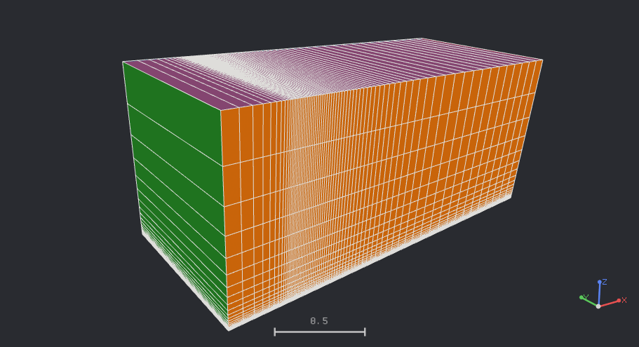
The `69×49` mesh in three dimensions — one cell in the spanwise direction; the plate is the bottom face, the upstream inlet is on the left, and the colors distinguish boundary groups

4.6 Boundary and Initial Conditions

Using a uniform farfield condition on the boundary-layer exit plane produces a near-wall pressure gradient. Therefore, a wind-tunnel-style domain uses the pressure_inlet/pressure_outlet combination. For the general definition of each boundary condition, see Domain and Boundary Conditions in the public Wake CFD documentation.

Boundary	Segment	Type	Setting
Wall	Plate, `x∈[0,2]`	`wall`	no-slip, adiabatic
Symmetry plane	Upstream slip segment + spanwise front/rear faces	`symmetry`	—
Inlet	Upstream	`pressure_inlet`	Total pressure `104190.6 Pa`, total temperature `302.4 K`, freestream `nu_tilde/nu = 3`
Outlet	Downstream	`pressure_outlet`	Back pressure `101325 Pa`
Farfield	Top	`farfield`	`Mach 0.2`, `101325 Pa`, `300 K`, freestream `nu_tilde/nu = 3`

Initial field: Not reported.

4.7 Numerical Methods

Item	Setting
Convergence criterion	Force-based — the drag and normal force coefficients each changing by less than `1×10⁻⁶` over 1,000 iterations. The `545×385` runs used a drag-only criterion (change below `1×10⁻⁸` over 1,000 iterations) and ended on an iteration cap and a manual stop, respectively, before it was met (see Convergence History)
Turbulence model	SA (Spalart–Allmaras) with the `ft2` term, `Pr_t = 0.9`
Convective scheme	Roe, no limiter, entropy fix off, `umuscl_kappa = 0.5`
Gradient method	Green–Gauss (`gg`) and weighted least squares (`wls`), each run on all five meshes (the selected method is also used for the viscous stresses and the SA terms)
Time integration	Euler implicit; FGMRES with DILU preconditioning (flow and turbulence)
CFL	Adaptive, `5 → 100` (reached `100` within about 20 iterations on all ten runs and stayed there)
Gas model	Ideal gas, `gamma = 1.4`, Sutherland viscosity (`S = 110.4 K`, reference viscosity set so that `Re_L = 5×10^6`), constant Prandtl number `0.72`

Note

Assumptions and differences from the references.

The TMR page and the CFL3D/FUN3D inputs specify only the reference temperature (540 °R = 300 K) and leave the viscosity law and the laminar Prandtl number to the codes’ defaults. Sutherland viscosity with Pr = 0.72 was assumed to match those defaults; this was not isolated, but the finest-mesh differences below are small.
The reference inputs differ from each other in the reconstruction setting: the CFL3D input uses RKAP0 = 0.33333 (kappa = 1/3), while FUN3D’s 2013 input uses kappa_umuscl = 0.5. Wake CFD was run with umuscl_kappa = 0.5.
The TMR page states that both reference codes advected the turbulence variable with first-order upwinding. Wake CFD also advects the turbulence variables with a first-order scheme, so this matches.
The TMR reference is the standard SA model (SA, with the ft2 term); the page notes that SA-noft2 gives essentially identical results for this case. The ft2 term was enabled in these runs.

For the general input structure and turbulence-model settings, see the CLI and Model Configuration sections of the public Wake CFD documentation.

4.8 Results

4.8.1 Convergence History

Eight of the ten runs converged by the force-based criterion. The iteration counts (Green–Gauss / weighted least squares) were 1,882 / 1,900 on 35×25, 2,797 / 2,787 on 69×49, 4,485 / 4,479 on 137×97, and 7,729 / 7,726 on 273×193. The two 545×385 runs did not end on the criterion and are described below (19,999 / 18,320 iterations in total, about 22.7 and 20.3 hours on 8 CPU cores).

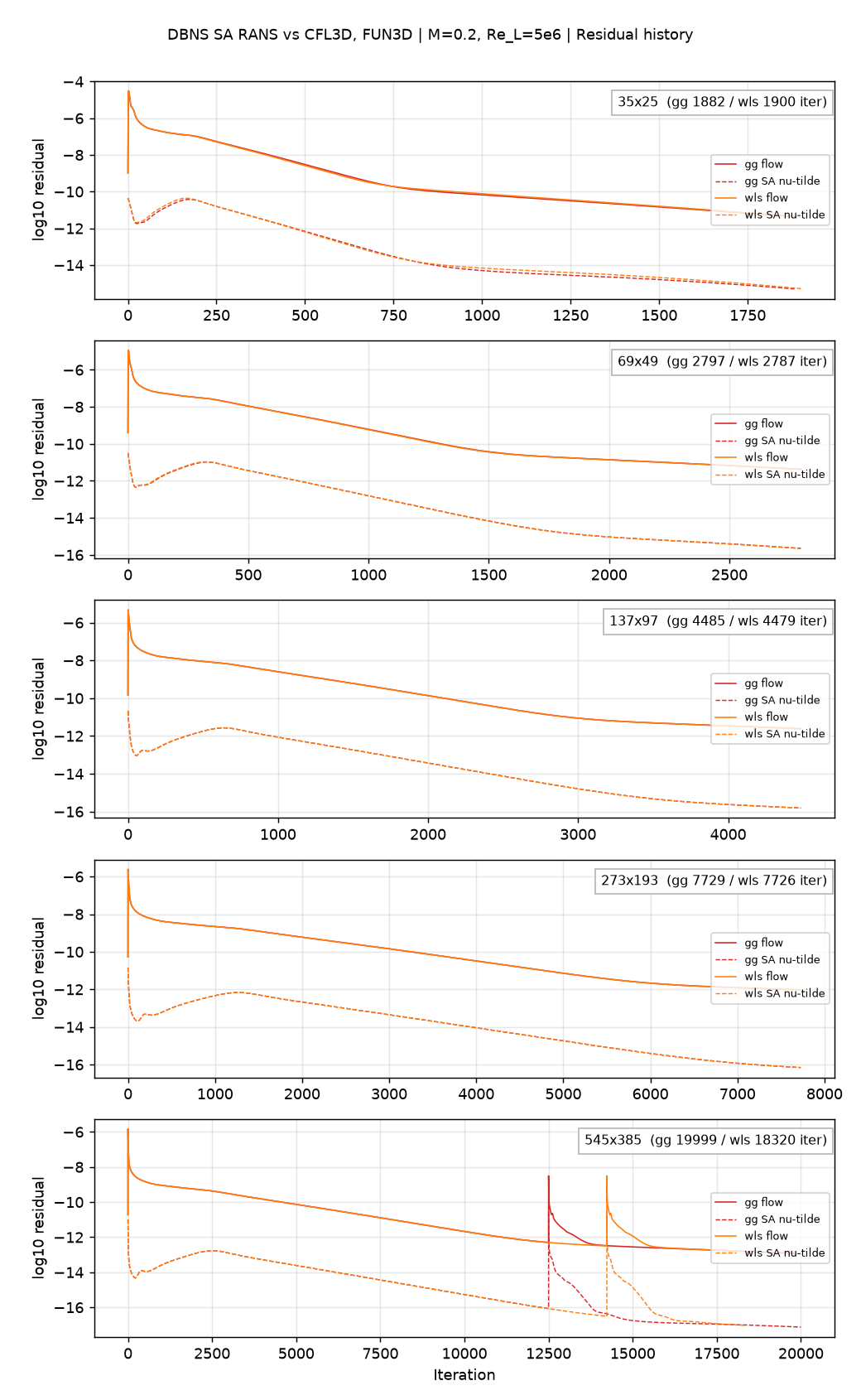
Residual history — absolute flow residual and SA `nu_tilde` residual, Green–Gauss and weighted least squares on each mesh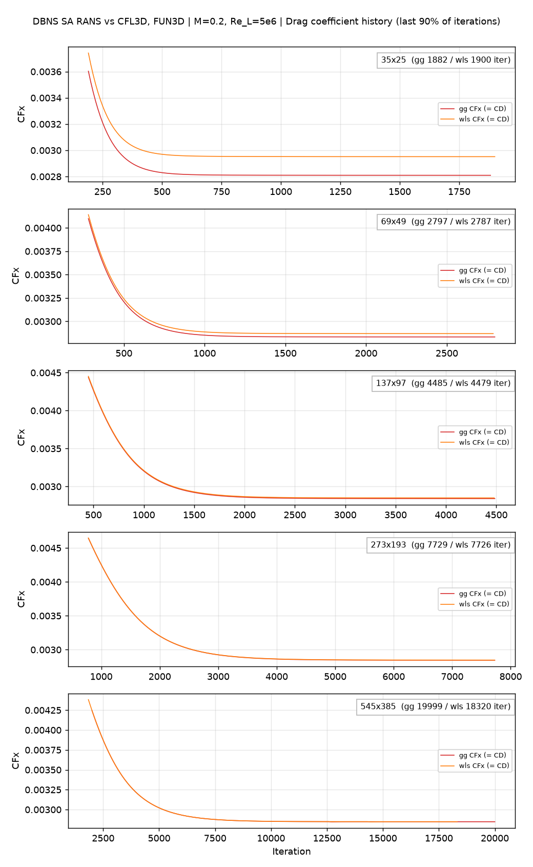

Drag-coefficient history on the five meshes (last 90% of the iterations)

The flow residual at termination was between -11.4 and -12.9 log10 (the termination criterion is force-based, not residual-based). The two gradient methods give residual and drag histories that are nearly indistinguishable on the three finest meshes.

The two 545×385 runs were stopped before reaching the criterion — the Green–Gauss run at the iteration cap (19,999) and the weighted-least-squares run manually at iteration 18,320. They are slightly less converged than the other eight: the drag coefficient was still drifting by about 0.002% per 1,000 iterations, more than an order of magnitude below the mesh-to-mesh differences and the offsets from the references discussed below. Because the two ended at different iteration counts, the C_D difference between the methods on this mesh carries an uncertainty of order 5×10⁻⁸ (at a common iteration, 18,320, it is 5.4×10⁻⁷).

4.8.2 Grid Convergence

The results were compared directly at the same mesh and station (x=0.970084) as the CFL3D/FUN3D data published by TMR.

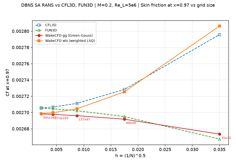
Grid convergence of `Cf(x=0.97)` — five Wake CFD points versus five CFL3D/FUN3D grid levels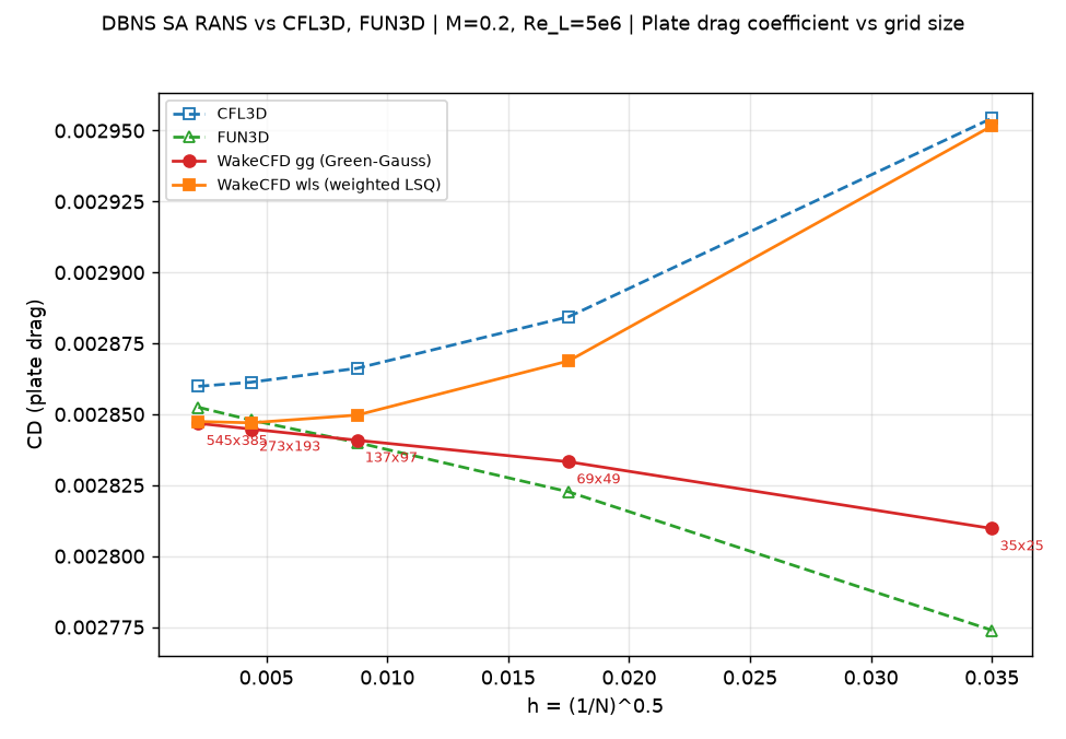

Grid convergence of the plate drag coefficient `C_D`

Both gradient methods are shown with the reference data. Cf is the skin-friction coefficient at x=0.97 and C_D is the plate drag coefficient.

Skin-friction coefficient at x=0.97:

Mesh	Wall `y+` (0.97)	`Cf` gg	`Cf` wls	CFL3D	FUN3D
35×25	1.51	0.002673	0.002806	0.002796	0.002667
69×49	0.74	0.002692	0.002725	0.002728	0.002695
137×97	0.37	0.002696	0.002704	0.002711	0.002702
273×193	0.18	0.002698	0.002700	0.002707	0.002704
545×385	0.09	0.002698	0.002699	0.002706	0.002705

Plate drag coefficient:

Mesh	`C_D` gg	`C_D` wls	CFL3D	FUN3D
35×25	0.002810	0.002952	0.002954	0.002774
69×49	0.002833	0.002869	0.002884	0.002823
137×97	0.002841	0.002850	0.002866	0.002840
273×193	0.002845	0.002847	0.002861	0.002848
545×385	0.002847	0.002847	0.002860	0.002852

Difference of Wake CFD relative to each reference code, on the same mesh:

Mesh	Method	`Cf` vs. FUN3D	`Cf` vs. CFL3D	`C_D` vs. FUN3D	`C_D` vs. CFL3D
35×25	gg	+0.23%	−4.37%	+1.29%	−4.90%
35×25	wls	+5.20%	+0.38%	+6.41%	−0.09%
69×49	gg	−0.12%	−1.34%	+0.38%	−1.77%
69×49	wls	+1.13%	−0.11%	+1.64%	−0.54%
137×97	gg	−0.22%	−0.56%	+0.03%	−0.89%
137×97	wls	+0.09%	−0.25%	+0.34%	−0.58%
273×193	gg	−0.25%	−0.34%	−0.11%	−0.58%
273×193	wls	−0.18%	−0.26%	−0.03%	−0.50%
545×385	gg	−0.26%	−0.27%	−0.20%	−0.46%
545×385	wls	−0.25%	−0.25%	−0.18%	−0.43%

On the finest mesh the two gradient methods give the same result (C_D 28.47 counts for both and Cf 26.98 / 26.99 counts of 1×10⁻⁴) and agree with both references within 0.46% (C_D) and 0.27% (Cf).
On coarse meshes the result depends strongly on the gradient method. At 35×25 the weighted-least-squares result is close to CFL3D (C_D −0.09%) and the Green–Gauss result is close to FUN3D (C_D +1.29%). The two references differ from each other by 6.5% in C_D there. The reason was not isolated; it is not a property of node-centered versus cell-centered discretization, since both Wake CFD runs use the same discretization apart from the gradient.
A systematic offset of about −0.25% in Cf relative to both references remains on the finest meshes for both gradient methods, and it does not shrink with refinement (Green–Gauss: −0.25% at 273×193 and −0.26% at 545×385). The two reference codes agree with each other to within 0.01% on the finest mesh, so this is not scatter between codes, and a discretization error would decrease with refinement. This points to a difference in setting or model between the Wake CFD runs and the references rather than a mesh effect. Candidates are the viscosity law (assumed, see above), umuscl_kappa, and the way Cf is extracted at the station; none has been isolated. The corresponding C_D difference is −0.20% (Green–Gauss) and −0.18% (weighted least squares) relative to FUN3D. The drift left at the end of the runs (about 0.002% per 1,000 iterations) is well below this offset.

4.8.3 Difference between the gradient methods

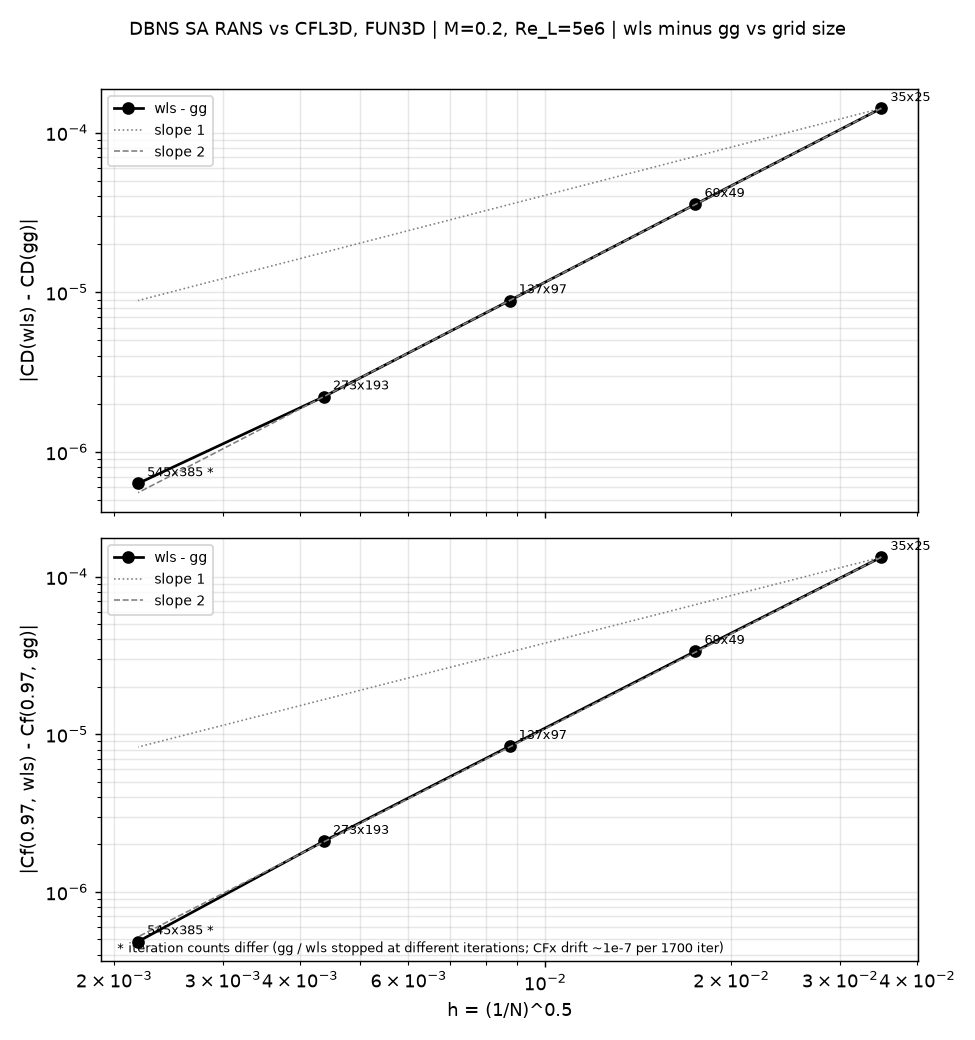
Difference between the weighted-least-squares and Green–Gauss results versus mesh size

The difference between the two methods drops by a factor of about four (h²) at each refinement:

Mesh	wls − gg, `C_D`	wls − gg, `Cf` (0.97)
35×25	1.419e-4	1.328e-4
69×49	3.557e-5	3.365e-5
137×97	8.868e-6	8.395e-6
273×193	2.215e-6	2.097e-6
545×385 (*)	6.3e-7	4.8e-7

(*) The two runs ended at different iteration counts (gg 19,999, wls 18,320), which adds an uncertainty of order 5×10⁻⁸ per 1,000 iterations. At the common iteration 18,320 the C_D difference is 5.4e-7. An h² extrapolation from the 273×193 row gives about 5.5e-7 (C_D) and 5.2e-7 (Cf).

Both methods therefore converge to the same solution, and the difference between them is a second-order term. All five points lie close to the slope-two line, including the 545×385 point, whose value carries an uncertainty of a few 10⁻⁷ from the residual drift (see Convergence History).

4.8.4 Observed order of convergence

The observed order p = log2(Δ_k / Δ_{k+1}) is computed from the changes Δ between successive meshes (each step halves the mesh spacing, so p = 2 means the change drops by a factor of four). The three values per row come from the three consecutive pairs of steps: 35→69→137, 69→137→273, and 137→273→545.

Code	Quantity	`p`
CFL3D	`C_D`	1.95 / 1.89 / 1.75
CFL3D	`Cf` (0.97)	1.97 / 1.96 / 1.98
FUN3D	`C_D`	1.49 / 1.14 / 0.80
FUN3D	`Cf` (0.97)	1.94 / 1.62 / 1.34
Wake CFD, gg	`C_D`	1.63 / 0.95 / 0.95 †
Wake CFD, gg	`Cf` (0.97)	2.08 / 1.50 / 1.28 †
Wake CFD, wls	`C_D`	2.12 / 2.81 / — ‡
Wake CFD, wls	`Cf` (0.97)	1.95 / 2.13 / 2.28

† The last value uses the 545×385 Green–Gauss run, which still drifts by about 0.0006 counts of 1×10⁻⁴ per 1,000 iterations (about 3% of the last C_D change), so digits beyond the first decimal are not reliable.

‡ The C_D change from 273×193 to 545×385 is +0.004 counts, with the opposite sign to the previous step, so p cannot be computed; it is of the same size as the residual drift.

CFL3D converges at second order throughout. The weighted-least-squares results behave like CFL3D over the first two steps (about second order) and the Cf values stay near second order on the finest step (the C_D step is within the noise). The Green–Gauss results and FUN3D both fall below second order on the fine meshes (about first order for C_D, between first and second for Cf). Both gradient methods use the same umuscl_kappa = 0.5 (CFL3D uses 1/3), so that setting alone cannot explain the lower order of the Green–Gauss results. The gradient method is a candidate, but this has not been tested directly. Because the order is below two for some codes, the finest-mesh values are not extrapolated with an h² law; the 545×385 values are the best available estimate of the grid-converged result rather than an extrapolated limit.

4.8.5 Detailed Comparison

The profiles below show the Wake CFD results (Green–Gauss and weighted least squares) against the CFL3D and FUN3D references (finest reference meshes). The profile figures use the 545×385 mesh.

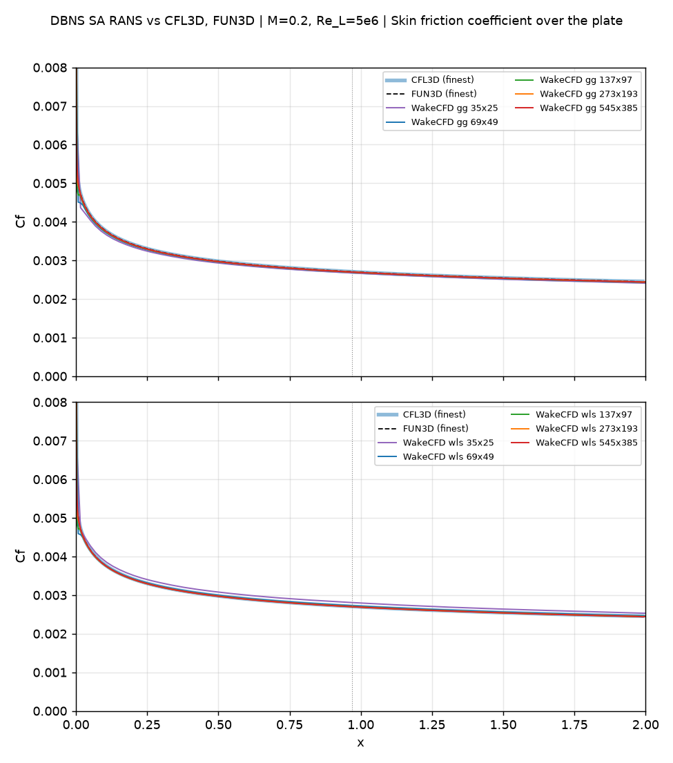
`Cf(x)` over the full plate on all five meshes for both gradient methods, against CFL3D and FUN3D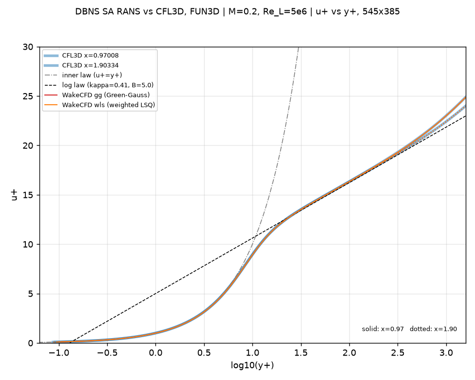

`u+` versus `y+` at x=0.97 (solid) and x=1.90 (dotted) against the law of the wall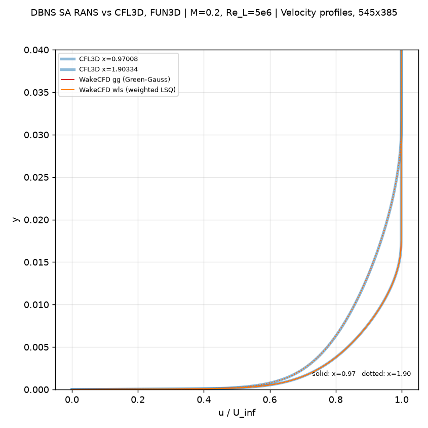

Velocity profiles `u/U_inf` versus height at x=0.97 and x=1.90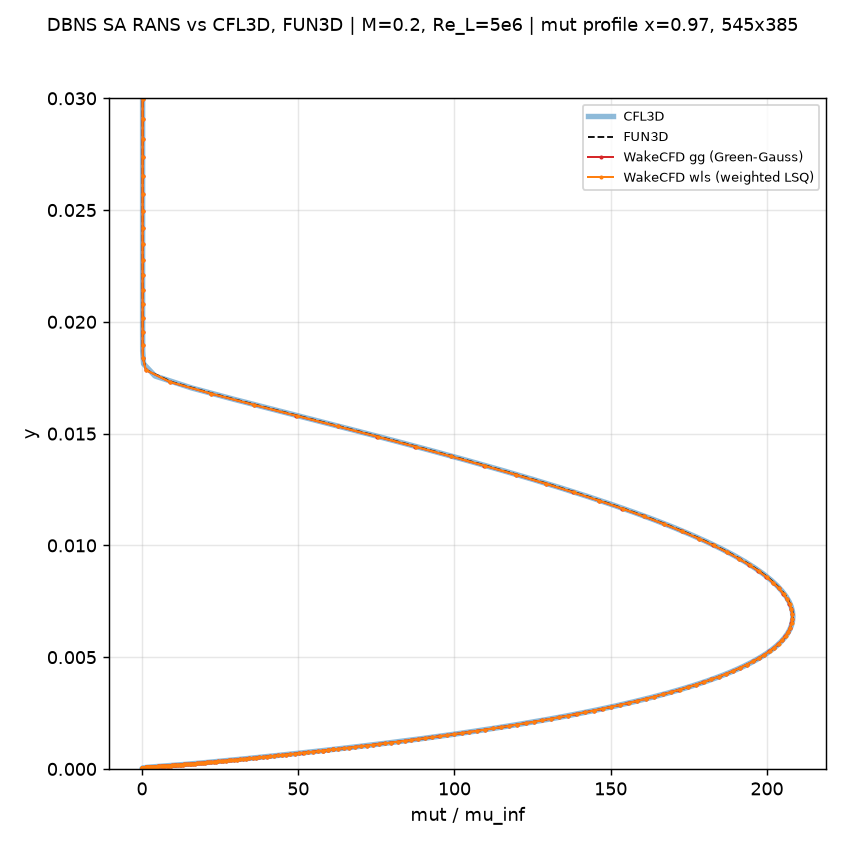

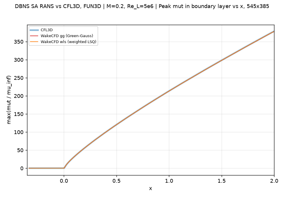
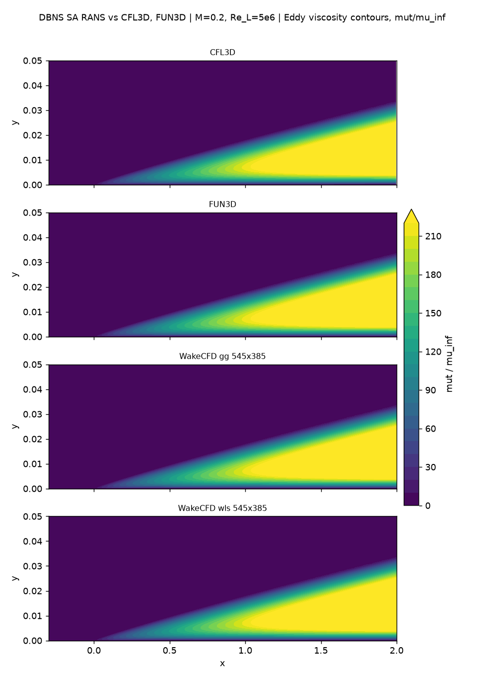
Maximum eddy-viscosity ratio in the boundary layer along the plate

Eddy-viscosity-ratio contours — CFL3D, FUN3D, and Wake CFD (both gradient methods) on the `545×385` mesh

Mesh	Max `mu_t/mu_inf` (0.97) gg / wls	Outer `u+` plateau (0.97) gg / wls
35×25	203.7 / 228.7	27.21 / 26.55
69×49	206.3 / 212.4	27.10 / 26.93
137×97	208.2 / 209.6	27.07 / 27.03
273×193	208.1 / 208.4	27.06 / 27.05
545×385	208.1 / 208.1	27.05 / 27.05
CFL3D (545×385)	208.3	27.05
FUN3D (545×385)	208.3	—
Finest-grid difference (vs. CFL3D / FUN3D)	−0.12% / −0.13% (gg), −0.08% / −0.09% (wls)	0.00%

On the finest meshes the peak eddy-viscosity ratio at x=0.97 is within 0.15% of the references for both gradient methods (Green–Gauss from 137×97, weighted least squares from 273×193), while the coarsest meshes deviate (−2.2% for Green–Gauss and +9.8% for weighted least squares at 35×25). The profile, the peak distribution along the plate, and the contours agree with both references. The u+ versus y+ curves follow the law of the wall through the viscous sublayer, the log region, and the outer plateau. The curves were compared visually; only the tabulated quantities above were quantified. The Cf offset of about −0.25% discussed above is not visible in these profile comparisons.

4.9 Conclusions and Applicable Scope

The SA turbulence-model implementation agrees with the official NASA TMR references (CFL3D and FUN3D) on the finest mesh within 0.46% for C_D and 0.27% for Cf, for both gradient methods, and within 0.15% for the peak eddy-viscosity ratio.
The full five-level grid-convergence family defined by TMR was run with both Green–Gauss and weighted-least-squares gradients. The two methods converge to the same solution, and the difference between them decreases as h². On coarse meshes the choice of method changes C_D by up to 5% at 35×25 and 1.3% at 69×49, so the method matters for coarse-mesh accuracy but not for the converged result.
A systematic difference of about −0.25% in Cf relative to both references remains for both gradient methods and does not shrink with refinement, so it is not a mesh effect. Its cause is not identified; candidates are the viscosity law, umuscl_kappa, and the extraction of Cf at the station.
The observed order of convergence of the weighted-least-squares Cf is close to two on all three steps, while the Green–Gauss results and FUN3D fall below second order on the fine meshes (Green–Gauss about first order for C_D). The cause of the lower order is not identified. The 545×385 runs ended on an iteration cap / manual stop with a small residual drift, so the finest-mesh values should be read as converged to within the differences in the tables above, not as extrapolated limits.
These results apply to a two-dimensional, zero-pressure-gradient flat plate at one subsonic condition (M=0.2). They cannot be generalized to pressure gradients, separation, transition, curved surfaces, or strong compressibility effects.
Follow-on validation should isolate the settings behind the remaining Cf offset, compare other RANS models (such as SST), and extend to pressure-gradient and fully three-dimensional geometries.

This case shows that Wake CFD’s SA turbulence-model implementation achieves accuracy comparable with mature reference codes for a subsonic flat-plate boundary layer without a pressure gradient. It establishes a minimum validation baseline for this range of conditions rather than an absolute accuracy guarantee.