3 2D Laminar Flat-Plate Boundary Layer — Blasius & Pohlhausen Verification
Verification of velocity profiles, wall friction, and wall heat transfer against the exact Blasius and Pohlhausen similarity solutions, across seven convective schemes
3.1 Run Provenance and Artifacts
| Item | Value |
|---|---|
| Wake CFD baseline version | 0.22.0 |
| Solver | DBNS |
| Compute device | CPU |
| Parallel execution | 1 MPI rank |
| Arithmetic precision | FP64 |
| Run date | 2026-09-20 |
Results depend on the solver build that produced them. Read every figure in this report together with the version and date above — re-running the same input on a later build may give different numbers.
3.1.1 Downloadable Files
Not available: input decks and result files have not yet been published for this case.
3.2 Verification Objective
This case simulates the boundary layer over a two-dimensional laminar flat plate and compares the computed result with the Blasius (velocity) and Pohlhausen (heat transfer) similarity solutions. It verifies Wake CFD implementation accuracy for:
- no-slip wall boundary conditions, both adiabatic-equivalent (Blasius) and isothermal (Pohlhausen)
- self-similarity of laminar boundary-layer velocity and temperature profiles
- variation of the local skin-friction coefficient (
Cf) and local Nusselt number (Nu_x) - low-Mach behavior of DBNS numerical fluxes, across seven convective schemes: five schemes with all-speed/low-Mach treatment (
AUSM+up,AUSM+up2,SLAU,SLAU2,Roe-Turkel) and two reference schemes without explicit low-Mach correction (Roe,JST)
Because the laminar flat-plate flow has zero pressure gradient and well-known analytical solutions for both the velocity and thermal boundary layers, it is a useful reference case for checking viscous-wall treatment, low-Mach schemes, numerical diffusion, and wall heat-flux computation together.
3.3 Reference Solution and Data
3.3.1 Analytical Solution
Let x be the distance from the leading edge, y the wall-normal distance, U_inf the freestream velocity, and nu the kinematic viscosity. The following nondimensional quantities are used:
\[ Re_x = \frac{U_\infty x}{\nu}, \qquad \eta = y\sqrt{\frac{U_\infty}{\nu x}}. \]
The Blasius solution is expressed as u/U_inf = f'(eta), with the primary comparison values:
\[ \delta_{99}\approx 4.91\sqrt{\frac{\nu x}{U_\infty}}, \qquad C_f(x)=\frac{0.664}{\sqrt{Re_x}}. \]
When velocity profiles at several x/L locations are plotted against eta, they should collapse onto a single curve.
For the thermal boundary layer, with an isothermal wall at temperature T_wall different from the freestream temperature T_inf, the Pohlhausen solution gives the local Nusselt number:
\[ Nu_x = \theta'(0)\sqrt{Re_x}, \qquad \theta'(0) = 0.295635 \text{ for } Pr=0.72, \]
where Pr is the Prandtl number. This case uses T_wall=327.38 K and T_inf=297.62 K with air (Pr≈0.72).
3.4 Simulation Conditions
| Item | Setting |
|---|---|
| Dimension | 2D |
| Domain | x=[0, 0.762] m, y=[0, 0.1524] m |
| Flat plate | x=[0.1524, 0.4572] m, L=0.3048 m |
| Analysis | Steady, compressible DBNS, laminar Navier–Stokes |
| Target Reynolds number | Re_L=1.0×10^5 |
| Mach conditions | 0.1, 0.05, 0.0144 |
| Wall | no-slip, isothermal, T_wall=327.38 K |
| Freestream temperature | T_inf=297.62 K (Pr≈0.72) |
To compare numerical behavior at low Mach numbers, viscosity was adjusted while keeping Re_L constant. Therefore, the Mach conditions do not all represent the same physical air experiment. M=0.0144 is a low-speed condition close to physical air viscosity; M=0.1 and M=0.05 compare low-Mach numerical behavior at the same Reynolds number.
3.5 Mesh
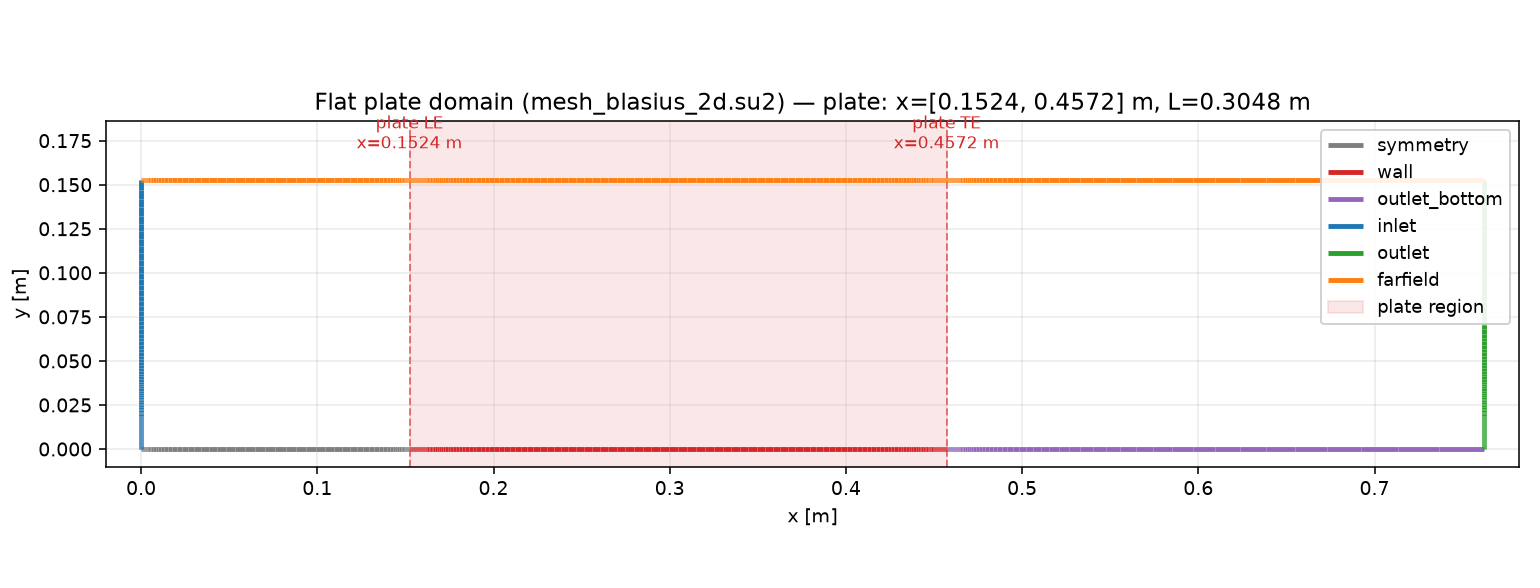
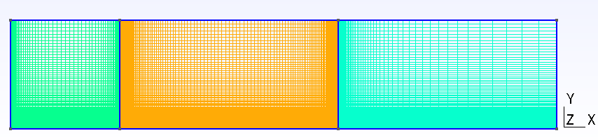
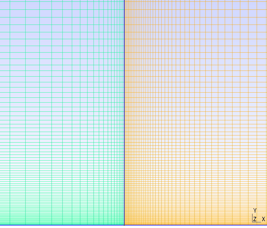
The computational domain consists of buffer regions upstream and downstream of the plate and a boundary-layer resolution region around it. The leading edge, trailing edge, and near-wall region are refined to capture boundary-layer velocity gradients and wall shear.
3.6 Boundary and Initial Conditions
| Boundary | Segment | Type | Setting |
|---|---|---|---|
| Wall | Plate segment | wall |
no-slip, isothermal |
| Symmetry plane | Bottom upstream of plate | symmetry |
— |
| Bottom outlet | Bottom downstream of plate | outlet_bottom |
— |
| Inlet | Left | inlet |
— |
| Outlet | Right | outlet |
— |
| Farfield | Top | farfield |
— |
Not reported: the source record does not specify the initial field for this steady-state calculation.
3.7 Numerical Methods
| Item | Setting |
|---|---|
| Analysis | Steady, compressible DBNS, laminar Navier–Stokes |
| Convective schemes | AUSM+up, AUSM+up2, SLAU, SLAU2, Roe-Turkel, Roe, JST (compared below) |
| Spatial accuracy | Second order, Venkatakrishnan limiter |
| Time integration | Euler implicit (steady solution) |
| CFL | Adaptive, 1 → 100 |
| Convergence criterion | Cauchy-window monitor on the total streamwise force coefficient CFx (eps=1e-5 over a 1000-iteration window) |
For the general input structure and boundary-condition definitions, see the CLI and Domain and Boundary Conditions sections of the public Wake CFD documentation.
3.7.1 Numerical Schemes Compared
Seven DBNS convective schemes were run at each of the three Mach numbers (21 cases total): five schemes designed for accuracy across a wide Mach range (AUSM+up, AUSM+up2, SLAU, SLAU2, Roe-Turkel, the last using a Turkel low-Mach preconditioner), and two reference schemes with no explicit low-Mach treatment (Roe, JST), included specifically to probe where low-Mach accuracy actually breaks down.
3.8 Results
3.8.1 Scheme comparison
| Method | Low-Mach treatment | Result summary (M=0.1 → 0.0144) |
|---|---|---|
| AUSM+up, AUSM+up2, SLAU, SLAU2 | All-speed flux formulation | Close to Blasius/Pohlhausen at every Mach; no degradation |
| Roe-Turkel | Turkel preconditioner | Close to Blasius/Pohlhausen at every Mach; converges in roughly 1/3–1/4 the iterations of the other schemes |
| Roe | None | Close to Blasius/Pohlhausen at every Mach — comparable to the all-speed group in this case |
| JST | None | Visibly degrades as Mach decreases; used here as the low-Mach control case |
These results do not imply that a particular flux scheme is superior for every problem; they show the applicable range of the numerical methods in Wake CFD for this specific flat-plate boundary layer, mesh, and Reynolds number. In particular, Roe remaining accurate down to M=0.0144 without explicit preconditioning is a case- and mesh-specific observation here, not a general claim about the scheme — see Conclusions below.
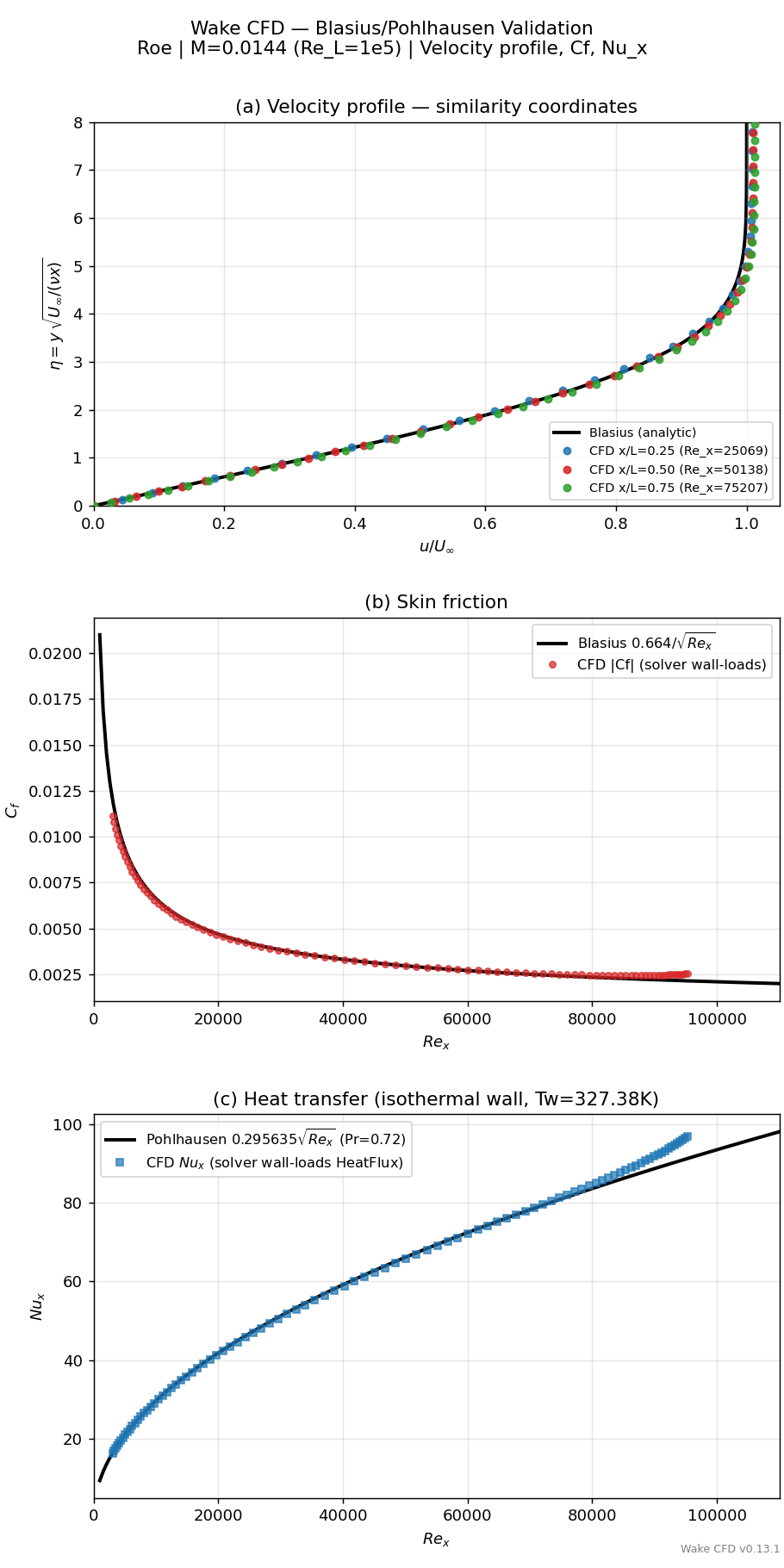
The comparison below aggregates all seven schemes at each Mach number. Two whole-plate metrics summarize accuracy at a glance: the mean ratio of computed skin friction to the Blasius reference, Cf/Cf_Blasius, and the mean ratio of computed local Nusselt number to the Pohlhausen reference, Nu_x/Nu_x,Pohlhausen, both averaged over x/L=0.03–0.95 (both are unweighted point-wise means, not force-integrated coefficients; ratios near 1.00 indicate agreement).
| Scheme | M |
Velocity RMS (x/L=.25,.50,.75) |
Cf/Cf_Blasius |
Nu_x/Nu_x,Pohlhausen |
|---|---|---|---|---|
| AUSM+up2 | 0.1 / 0.05 / 0.0144 | 0.7–1.1% at all three | 1.02–1.03 | 0.98 → 1.00 |
| AUSM+up | 0.1 / 0.05 / 0.0144 | 0.7–1.1% at all three | 1.02–1.03 | 0.98 → 1.00 |
| SLAU2 | 0.1 / 0.05 / 0.0144 | 0.7–1.1% at all three | 1.02–1.03 | 0.98 → 1.00 |
| SLAU | 0.1 / 0.05 / 0.0144 | 0.7–1.1% at all three | 1.02–1.03 | 0.98 → 1.00 |
| Roe-Turkel | 0.1 / 0.05 / 0.0144 | 0.7–1.0% at all three | 1.02 | 0.98 → 1.00 |
| Roe | 0.1 / 0.05 / 0.0144 | 0.7–1.1% at all three | 1.02 | 0.98 → 1.01 |
| JST | 0.1 / 0.05 / 0.0144 | 1.0–1.2% → 2.2–3.3% | 1.09 → 1.16 | 0.99 → 1.02 |
For all seven schemes, Nu_x moves monotonically closer to the Pohlhausen value as M decreases (from roughly −2% at M=0.1 to within +0.5% at M=0.0144); this trend is consistent with a compressible, ideal-gas isothermal-wall coupling that vanishes as M→0, since the analytical Pohlhausen solution assumes constant properties. Six of the seven schemes hold their velocity/Cf accuracy essentially flat across the whole Mach range; only JST shows a clear, monotonic degradation, concentrated in the second half of the plate where the boundary layer is thinnest and wall-normal gradients are largest.
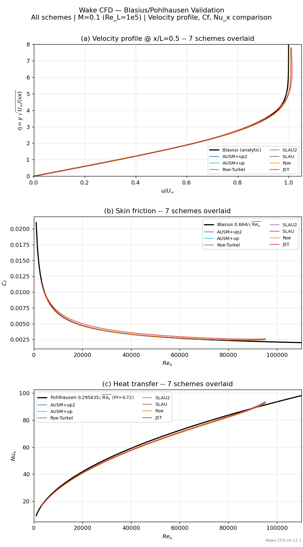
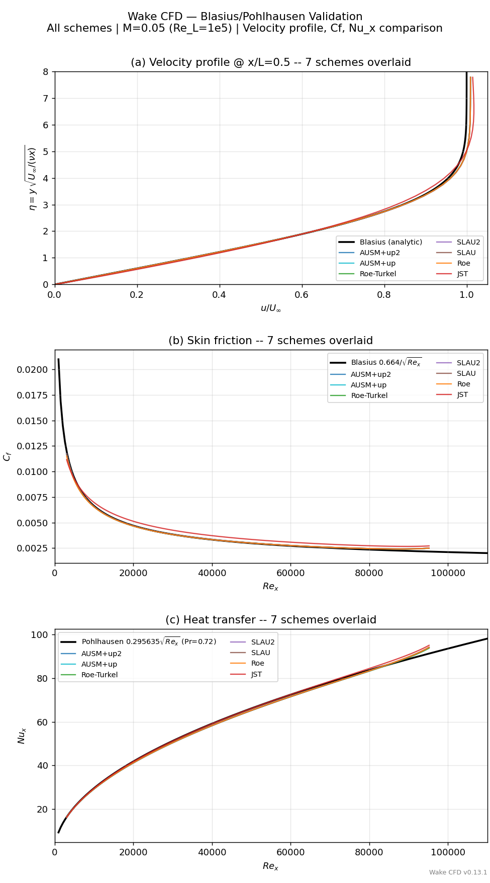
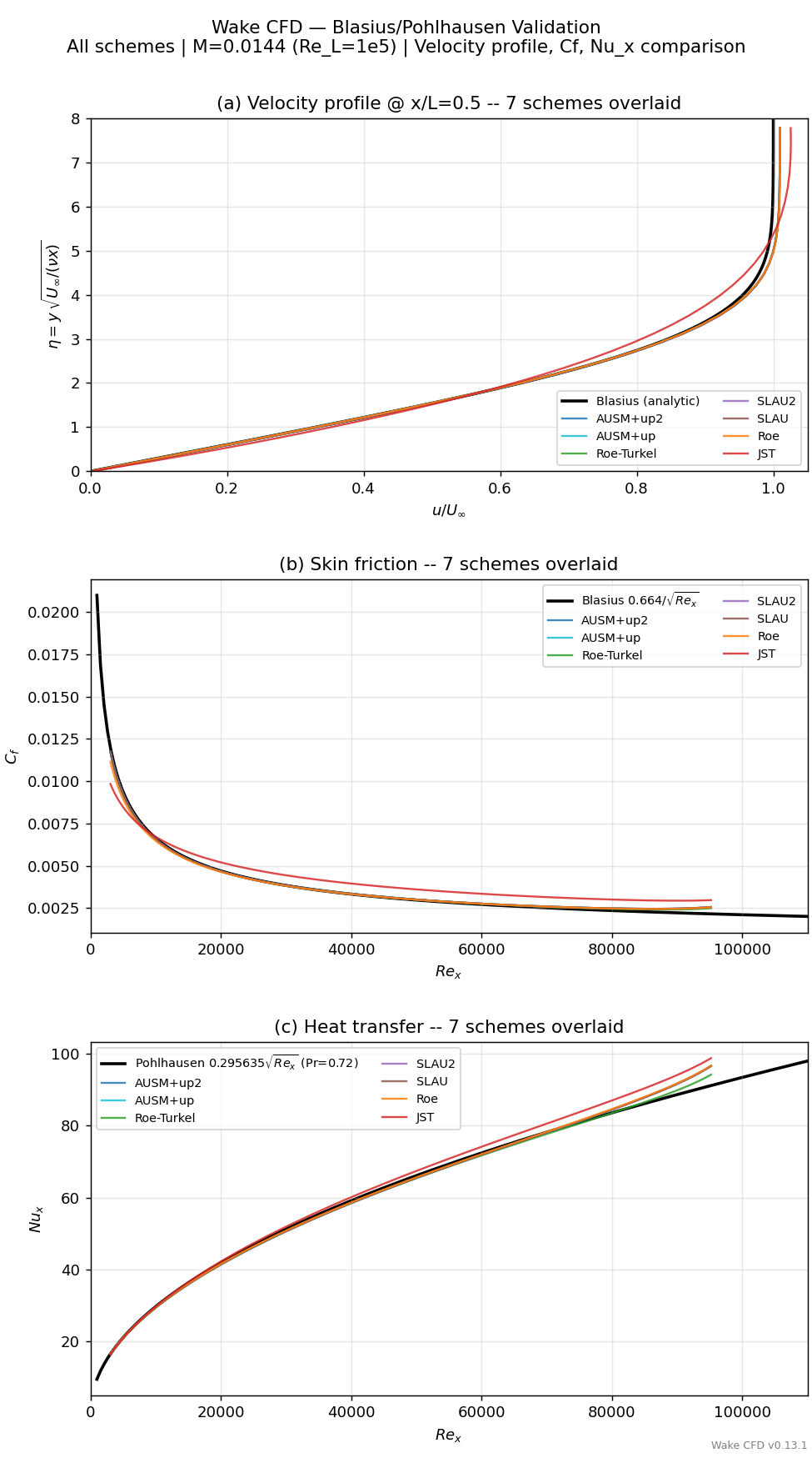
At M=0.1 all seven curves are essentially indistinguishable. As Mach decreases, JST (shown in red) separates visibly from the rest, while the five all-speed schemes and Roe remain clustered on the reference curves even at M=0.0144.
3.8.2 Closer Look: Roe Without Low-Mach Preconditioning
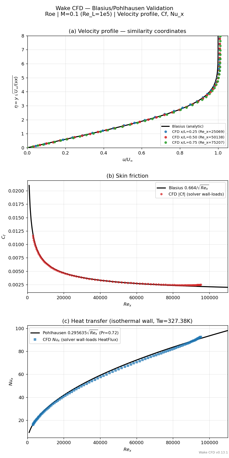
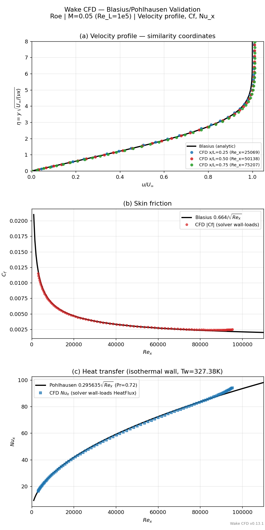
Roe is highlighted separately because, unlike JST, it was not expected to hold its accuracy at low Mach without an explicit correction (compare Roe-Turkel, which adds a Turkel preconditioner to the same base scheme). The station-by-station detail below is the same comparison used to build the summary table above, shown per Mach with all three stations (x/L=0.25, 0.50, 0.75) instead of the single-station overlay.
M |
Velocity RMS (x/L=.25,.50,.75) |
δ99(η) (x/L=.25,.50,.75) |
Cf/Cf_Blasius |
Nu_x/Nu_x,Pohlhausen |
|---|---|---|---|---|
| 0.1 | 0.68%, 0.67%, 0.96% | 4.71, 4.61, 4.49 | 1.021 | 0.981 |
| 0.05 | 0.70%, 0.70%, 0.99% | 4.70, 4.60, 4.49 | 1.021 | 0.995 |
| 0.0144 | 0.78%, 0.72%, 1.06% | 4.71, 4.59, 4.47 | 1.022 | 1.005 |
(The Blasius reference value of δ99(η) is approximately 4.9.)
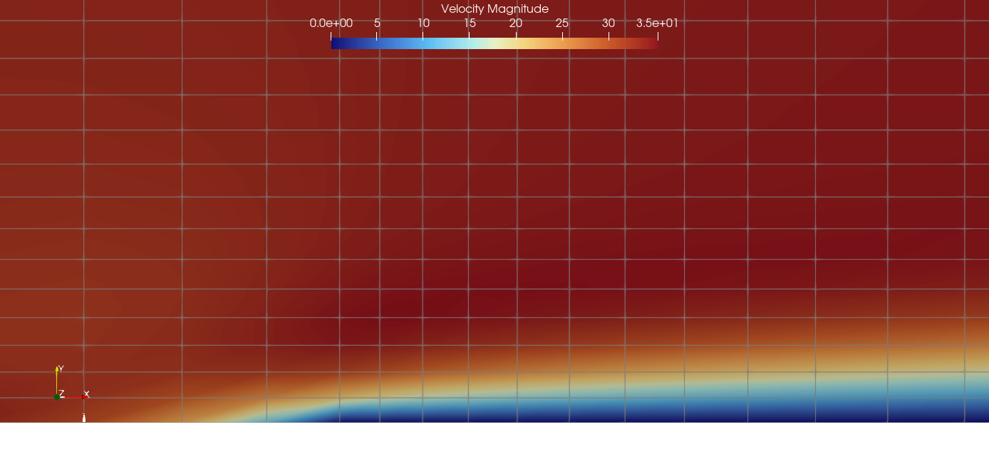
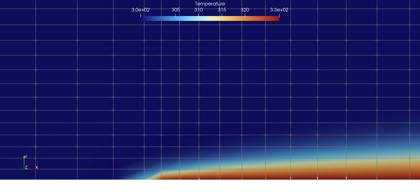
For qualitative reference, the two contour plots below (M=0.1) show the velocity and temperature fields near the leading edge, illustrating the developing momentum and thermal boundary layers on the isothermal wall.
3.9 Conclusions and Applicable Scope
- The five all-speed schemes (
AUSM+up,AUSM+up2,SLAU,SLAU2,Roe-Turkel) agree well with both the Blasius velocity profile and the Pohlhausen heat-transfer solution fromM=0.1down toM=0.0144, and are essentially indistinguishable from one another on this case. Roe-Turkelreaches its converged state in roughly 1/3–1/4 the iterations of the other six schemes at the same Mach numbers; its practical advantage here is convergence speed rather than accuracy.JST, run without low-Mach correction as a control case, shows the expected monotonic loss of accuracy as Mach decreases, confirming that some form of low-Mach treatment is needed for schemes of this type on this problem.Roe, also run without explicit low-Mach correction, unexpectedly remained close to the all-speed group down toM=0.0144on this mesh and Reynolds number. This should not be read as a general claim thatRoedoes not need low-Mach treatment — it has not been checked at other mesh densities, Reynolds numbers, or geometries, and is reported here as an observation specific to this case.- These results apply only to a 2D, steady, laminar flat-plate boundary layer at
Re_L=1×10^5. They cannot be generalized to turbulence, pressure gradients, curved surfaces, separation, transition, or other Reynolds numbers. - Follow-on validation should vary mesh resolution, Reynolds number, and wall-temperature ratio independently to check whether the
Roe/JSTsplit observed here persists.
This case does not establish absolute accuracy of the Wake CFD solver. It defines minimum applicable numerical-analysis conditions for a low-Mach viscous-wall problem, with and without wall heat transfer, with zero pressure gradient on a two-dimensional geometry.
3.10 References
- Blasius, H., “Grenzschichten in Flüssigkeiten mit kleiner Reibung,” Zeitschrift für Mathematik und Physik, 56, 1908, pp. 1–37.
- Pohlhausen, E., “Der Wärmeaustausch zwischen festen Körpern und Flüssigkeiten mit kleiner Reibung und kleiner Wärmeleitung,” Zeitschrift für Angewandte Mathematik und Mechanik, 1, 1921, pp. 115–121.
- White, F.M., Viscous Fluid Flow, 3rd ed., McGraw-Hill, 2006 (Blasius and Pohlhausen similarity solutions, Chapter 4).