19 2D Transonic Airfoil — RAE2822 RANS Validation
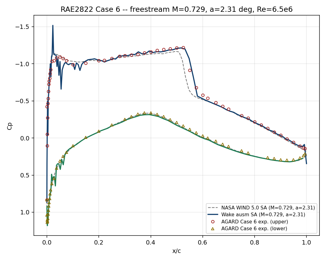
Comparison of shock location and surface pressure distribution against the AGARD Case 6 experiment
19.1 Run Provenance and Artifacts
| Item | Value |
|---|---|
| Wake CFD baseline version | 0.22.2 |
| Solver | DBNS |
| Compute device | CPU |
| Parallel execution | 1 MPI rank |
| Arithmetic precision | FP64 |
| Run date | 2026-08-18 |
Results depend on the solver build that produced them. Read every figure in this report together with the version and date above — re-running the same input on a later build may give different numbers.
19.1.1 Downloadable Files
Not available: standalone input decks and solver result files have not yet been published for download.
19.2 Validation Objective
For a transonic airfoil, small changes in conditions can substantially alter the shock location and lift. This case compares the surface pressure distribution of the widely used RAE2822 airfoil with experiment to establish the range over which Wake CFD reproduces two-dimensional transonic turbulent flow with a shock.
For users, this result supports review of airfoil pressure distributions, shock locations, and lift levels during early design. In particular, the default Roe scheme reproduces both the suction-side shock and lift level observed in experiment.
19.3 Reference Solution and Data
| Item | Setting |
|---|---|
| Reference | AGARD AR-138 RAE2822 Case 6 pressure distribution and lift (C_L=0.743) |
19.4 Simulation Conditions
| Item | Setting |
|---|---|
| Geometry | RAE2822 2D airfoil |
| Analysis | Steady, compressible RANS |
| Freestream Mach | 0.729 |
| Angle of attack | 2.31° |
| Reynolds number | Re_c=6.5×10^6 |
| Reference temperature | 288.15 K |
This setup uses the free-air-corrected condition for AGARD Case 6. The Case 9 pressure data in the same data set use a different angle of attack and lift level, and therefore are not compared directly with the Case 6 result. Checking the case number for both conditions and experimental data is essential when reproducing this case.
19.5 Mesh
| Item | Setting |
|---|---|
| Mesh | 2D C-mesh, 192 points on the airfoil surface |
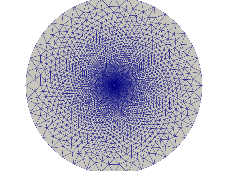
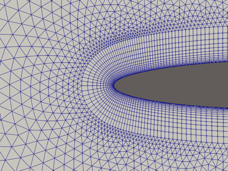
The baseline mesh is a 2D C-mesh with 192 points on the airfoil surface, comprising 13,937 nodes and 22,842 elements. The airfoil surface and near field where the shock forms are refined, with progressively coarser spacing toward the farfield.
19.6 Boundary and Initial Conditions
N/A: Detailed boundary and initial conditions are not documented for this case.
19.7 Numerical Methods
| Item | Setting |
|---|---|
| Turbulence model | Spalart–Allmaras (SA) |
| Convective schemes | Roe, HLLC, JST, AUSM+up, AUSM+up2, SLAU, SLAU2, and AUSM (compared below) |
Time integration and convergence settings: Not reported.
19.8 Results
19.8.1 Key Results
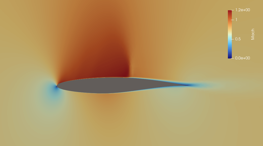
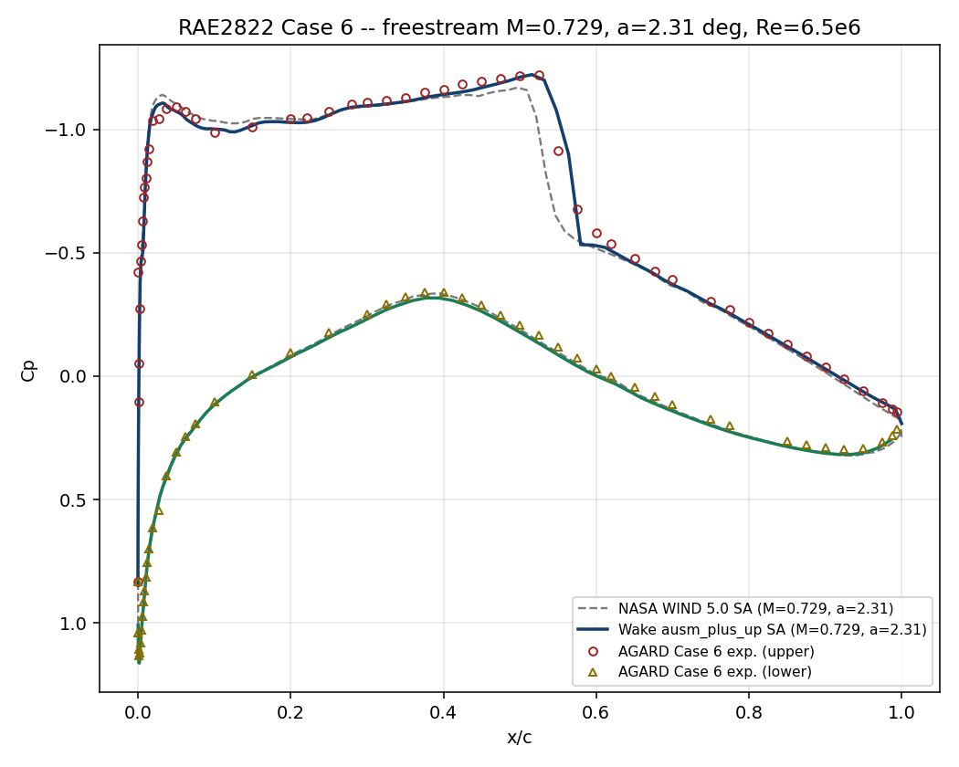
The baseline Roe configuration converged in 4,697 iterations and predicted C_L=0.7455, a 0.3% difference from the Case 6 experimental value of 0.743. The suction-side shock was also captured near the experimental location, x/c≈0.55.
The Mach contour shows the flow accelerating over the suction side to form a local supersonic region, followed by sharp compression near x/c≈0.55. The pressure-coefficient contour likewise shows a distinct pressure recovery at the same location, consistent with the shock location identified in the surface pressure comparison.
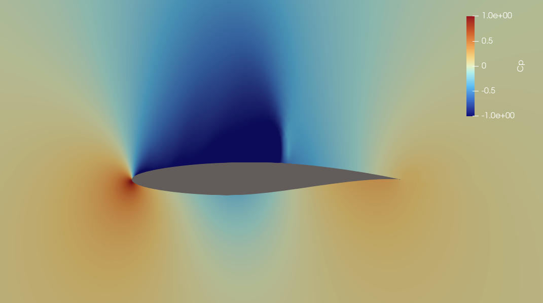
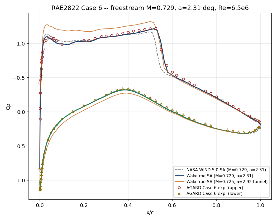
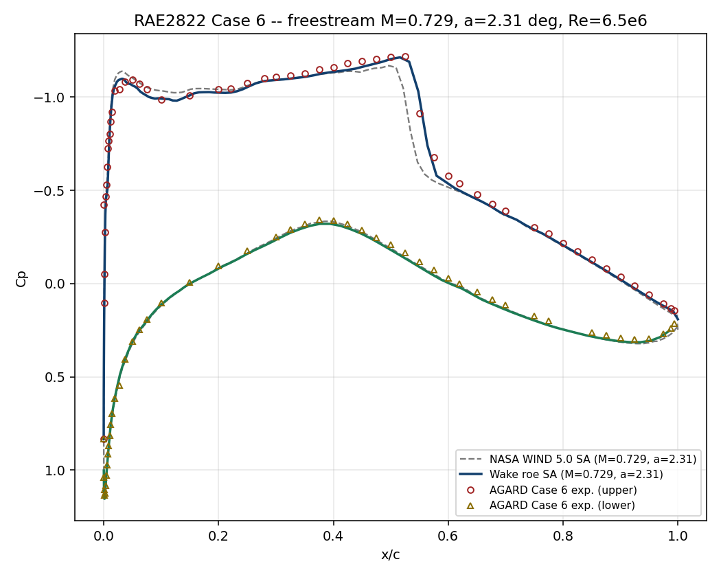
The pressure-distribution shape on both sides of the shock and the pressure recovery agree well overall with the experimental points. Because interpolation near the sharp leading-edge pressure variation can make RMS error appear large, this case considers shock location, pressure-distribution shape, and lift coefficient together.
19.8.2 Comparisons for Scheme Selection
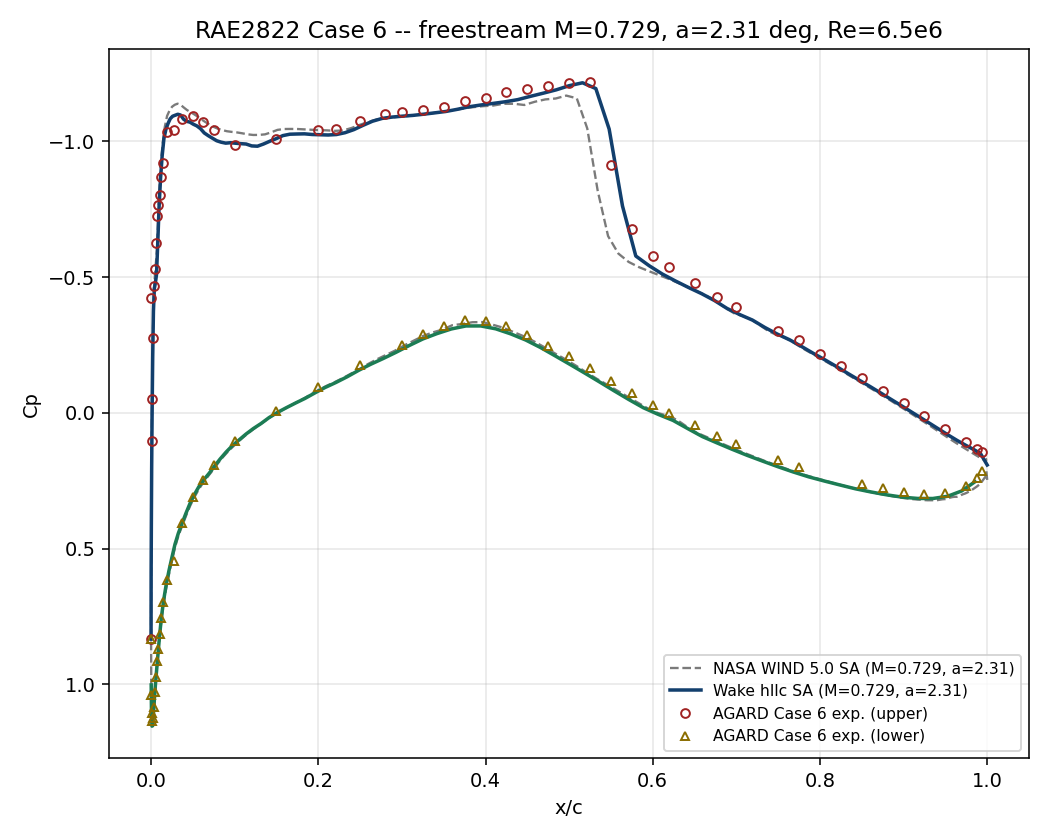
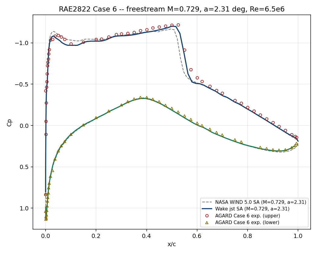
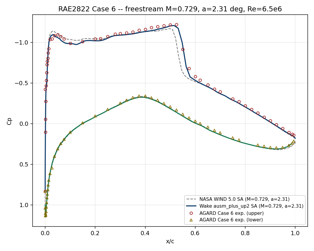
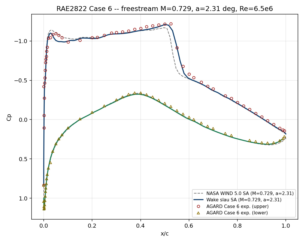
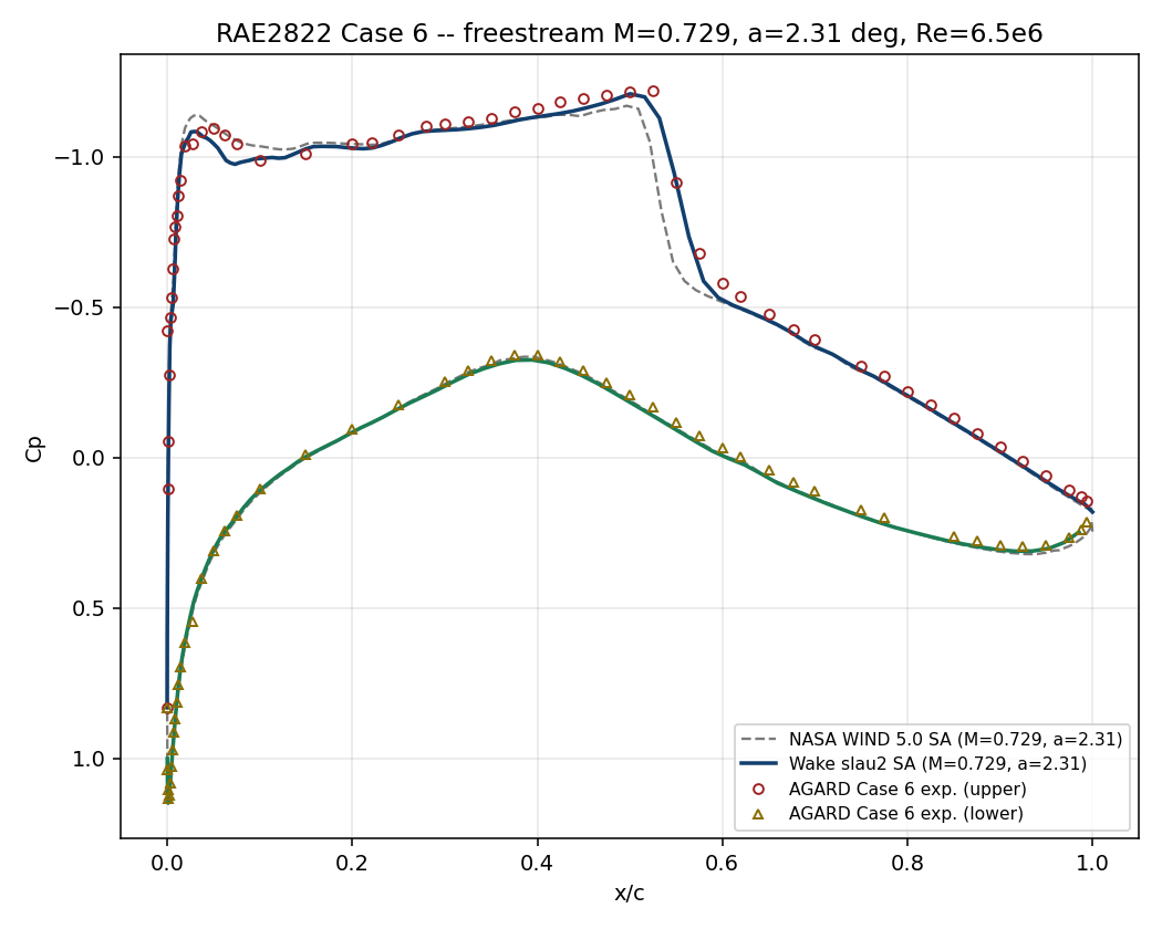
Only the convective scheme was varied while keeping the mesh and turbulence model fixed. The pressure distribution is reproduced similarly by several schemes, but reaching the target convergence is as important as accuracy in practice.
| Scheme | Lift coefficient | Iterations | Convergence status | Assessment |
|---|---|---|---|---|
| Roe | 0.7455 | 4,697 | Converged | Default choice |
| HLLC | 0.7471 | 4,693 | Converged | Roe alternative |
| JST | 0.7266 | 5,205 | Converged | Usable |
| AUSM+up | 0.7564 | 4,663 | Converged | Usable |
| AUSM+up2 | 0.7383 | 4,712 | Converged | Usable |
| SLAU / SLAU2 | 0.7404 / 0.7385 | 20,000 | Residual stagnation* | Further tuning required |
| AUSM | 0.7589 | 20,000 | Leading-edge oscillation | Not recommended |
* The pressure distribution and force coefficients stabilized, but the specified residual-reduction criterion was not reached.
19.9 Conclusions and Applicable Scope
- Roe is recommended as the default scheme for this condition. It gives the closest lift to experiment and reaches the specified convergence criterion robustly.
- If an alternative is required, consider HLLC, JST, AUSM+up, or AUSM+up2. All reproduced the shock and pressure distribution stably in this case.
- Plain AUSM produced leading-edge pressure oscillations. SLAU/SLAU2 did not reach the target residual without additional CFL or linear-solver tuning.
- This result validates one airfoil, one Reynolds number, and a two-dimensional steady RANS condition. It does not guarantee the same accuracy for a real three-dimensional wing, transition or separation, unsteady buffet, other turbulence models, or other mesh quality.
19.10 References
- Cook, P. H., McDonald, M. A., Firmin, M. C. P., Aerofoil RAE 2822 — Pressure Distributions, and Boundary Layer and Wake CFD Measurements, AGARD AR-138, 1979.
- NASA NPARC Alliance RAE2822 Verification & Validation Archive