20 Numerical methods

DBNS, PBNS, FR, CFL, time integration, and linear solvers

20.1 What this setting is

Numerical methods determine how the selected equations are discretized and solved. Start with analysis.solver, then read the corresponding block below. Each table explains where a knob belongs, when it is active, and what changing it affects. Change one numerical setting at a time and compare residuals and the quantities you monitor.

numerical_method contains numerical options activated by analysis.solver. Do not mix solver-specific blocks with the linear solver shared by DBNS and PBNS.

20.2 Configure in the GUI

The Desktop editor covers the DBNS route through four tabs. The dialog says so in its header: PBNS and FR editors are not yet available, so those solvers are configured in JSONC. CFL belongs to Run Control, matching its run_control location in the deck, and therefore does not appear here.

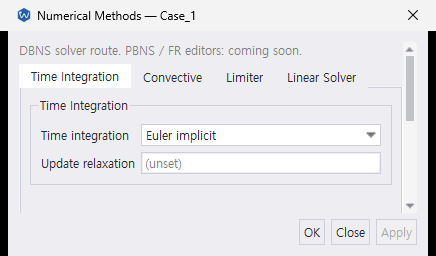
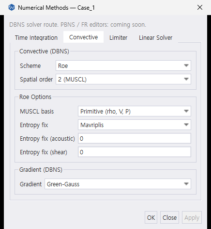
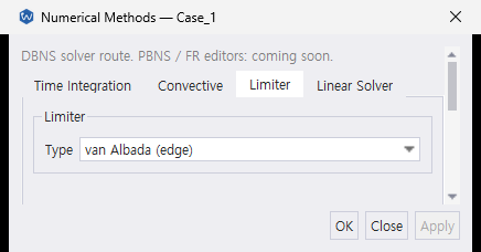
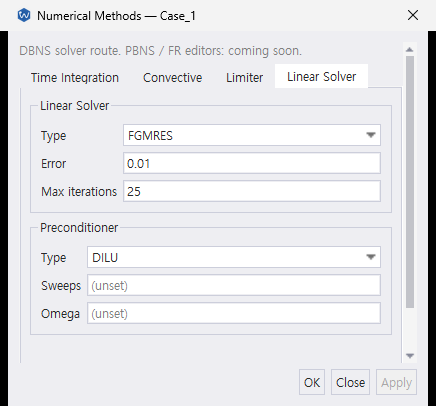
Numerical Methods dialog, Time Integration tab, with Euler implicit selected and an unset update relaxation — (a) **Time Integration** — the pseudo-time scheme.

Numerical Methods dialog, Convective tab, with Roe flux, second-order MUSCL, primitive MUSCL basis, Mavriplis entropy fix, and Green-Gauss gradient — (a) **Time Integration** — the pseudo-time scheme.

Tab	GUI control	Input key
Time Integration	Time integration	`numerical_method.dbns.time_integration`
Time Integration	Update relaxation	`numerical_method.dbns.nonlinear.relaxation`
Convective	Scheme	`numerical_method.dbns.convective.scheme`
Convective	Spatial order	`numerical_method.dbns.convective.spatial_order`
Convective	MUSCL basis	`numerical_method.dbns.convective.roe.reconstruction`
Convective	Entropy fix	`numerical_method.dbns.convective.roe.entropy_fix_type`
Convective	Entropy fix (acoustic) / (shear)	`…roe.entropy_fix_acoustic`, `…roe.entropy_fix_shear`
Convective	Gradient	`numerical_method.dbns.gradient`
Limiter	Type	`numerical_method.dbns.convective.limiter.type`
Linear Solver	Type / Error / Max iterations	`numerical_method.linear_solver.{type, error, max_iter}`
Linear Solver	Preconditioner Type / Sweeps / Omega	`numerical_method.linear_solver.preconditioner.flow.{type, sweeps, omega}`

The scheme-specific box under Convective is refilled when the scheme changes, so the Roe options above appear only while roe is selected. The Preconditioner box edits the flow block; the turb, energy, and solid blocks are JSONC-only.

20.3 Configure in JSONC

Solver	Active block	Purpose
`dbns`	`numerical_method.dbns`	Density-based FVM
`pbns`	`numerical_method.pbns`	Pressure-based 3D solver
`fr`	`numerical_method.fr`	Flux Reconstruction, unsteady only
`dbns`, `pbns`	`numerical_method.linear_solver`	Shared settings for implicit linear systems

Do not use legacy examples of generic numerical_method.convective based on analysis.discretization as a reference for the current input structure.

20.4 Where step-size knobs live

Physical-time schemes, stopping limits, and pseudo-time policies are explained in Run control and convergence. They are separate from the numerical-method blocks on this page:

Solver	Step-size knob	When it applies
DBNS	`run_control.cfl`	Steady pseudo-time, unsteady dual-time inner iterations, or physical Δt with `standard` explicit stepping.
PBNS	`run_control.pseudo_time`	Steady pseudo-time only.
PBNS	`numerical_method.pbns.timestep.cfl_acoustic`, `.cfl_flow`, `.cfl_diffusion`	Caps on the evolving physical Δt in unsteady analysis.
FR	`run_control.pseudo_time`	Dual-time inner iterations.
FR	`run_control.timestep_control`	Adaptive physical Δt for explicit `rk34`/`rk45`.

Warning

For a PBNS case, putting CFL under run_control.cfl is silently ignored — that’s the DBNS axis — and PBNS runs with its unset default. Use run_control.pseudo_time for steady analysis or pbns.timestep.cfl_acoustic/cfl_flow/cfl_diffusion for unsteady analysis.

20.5 DBNS

20.5.1 Convective terms

{
  "numerical_method": {
    "dbns": {
      "convective": {
        "scheme": "roe",
        "spatial_order": 2,
        "limiter": { "type": "venkatakrishnan", "coeff": 0.3 }
      }
    }
  }
}

The first decision is the convective flux. Put scheme-specific keys such as jacobian, Roe entropy fix, and JST ad_coeff in the subblock named for the selected scheme. The keys in this table live under numerical_method.dbns.convective unless a different path is shown.

Key	Values / default	What it controls
`scheme`	`jst`, `roe`, `ausm`, `ausm_plus_up`, `ausm_plus_up2`, `hllc`, `slau`, `slau2`	Numerical flux at cell faces. Change it when comparing shock capture, dissipation, or low-Mach behavior. `roe_turkel` is a scheme of its own, not an option of `roe`.
`spatial_order`	`1` or `2`	First-order reconstruction or second-order MUSCL reconstruction. Second order uses the reconstruction gradient and limiter.
`limiter.type`	`none`, `venkatakrishnan`, `barth`, `nishikawa_r3`, `venkatakrishnan_wang`, `van_albada_edge`	Bounds the second-order reconstruction near steep gradients. `none` removes this bound; `van_albada_edge` limits each edge separately.
`limiter.coeff`	`0.05` in the input reference	Venkatakrishnan limiter strength: a larger value weakens limiting. Ignored by `van_albada_edge`.
`limiter.elem_length`	`0.1` m in the input reference	Characteristic mesh length used with `limiter.coeff`; choose a representative mesh scale when using the Venkatakrishnan limiter. Ignored by `van_albada_edge`.
`limiter.freeze_iter`	`-1` (disabled)	Positive outer iteration after which the nodal limiter stops updating. JFNK also freezes it when Newton activation begins. Ignored by `van_albada_edge`.
`umuscl_kappa`	`0.0`; allowed `[-1, 1)`	Mean-flow U-MUSCL face bias. Keep the default unless comparing reconstruction schemes; turbulence reconstruction is unaffected.

numerical_method.dbns.gradient is the physical gradient. A separate convective.reconstruction_gradient changes only MUSCL reconstruction:

Key	Default	What it controls
`dbns.gradient`	`weighted_least_squares`	Physical gradient for viscous fluxes, turbulence, derived fields, and (unless overridden) MUSCL. Choose `weighted_least_squares` or `green_gauss`; unweighted `least_squares` is not accepted here.
`convective.reconstruction_gradient`	Reuses `dbns.gradient`	MUSCL gradient only: `weighted_least_squares`, `green_gauss`, or `least_squares`. The unweighted choice is rejected with JST and first-order reconstruction.

Omitting reconstruction_gradient reuses the physical gradient and avoids a second gradient field. For umuscl_kappa, 0.0 is the current upstream-biased second-order form; changing it alters the face state and should be evaluated against the same mesh and convergence target.

{
  "numerical_method": {
    "dbns": {
      "gradient": "weighted_least_squares",
      "convective": {
        "scheme": "roe",
        "roe": {
          "entropy_fix_type": "mavriplis",
          "entropy_fix_acoustic": 0.001,
          "entropy_fix_shear": 0.0,
          "jacobian": "roe_exact"
        }
      }
    }
  }
}

Key	Meaning
`entropy_fix_type`	`harten_hyman` or `mavriplis`
`entropy_fix_acoustic`	Acoustic-wave entropy fix; default `0.0` (off).
`entropy_fix_shear`	Contact/shear-wave fix; default `0.0`. Use for strong-shock carbuncle control, not as a general wall-flow adjustment.
`reconstruction`	`primitive` (default) or `eos` for Roe-family MUSCL face states. The EOS option derives face density from extrapolated pressure and temperature; validate shock convergence before changing it.
`jacobian`	`scalar_dissip`, `roe_exact`, `hllc_exact`, `ausm_ad`, `ausm_fd`, or `turkel_exact`. Default `roe_exact`; `convective.roe_turkel.jacobian` has the same values and defaults to `turkel_exact`

JFNK freezes the nodal limiter when Newton activation begins so its matrix-free linear operator stays fixed. van_albada_edge has no stored nodal limiter, so its coeff, elem_length, and freeze_iter keys are ignored.

20.5.2 Low-Mach dissipation and time stepping

Low-Mach treatment is one block. Select scheme: "roe_turkel" for the preconditioned dissipation, and set the single β that the dissipation, the preconditioned time step, and the Γ⁻¹ term all share in numerical_method.dbns.low_mach.

The reference Mach number M_ref is max(freestream Mach, reference.velocity / freestream sound speed). Supply a representative speed in reference.velocity for a hovering rotor, such as tip speed.

All four keys below are inside numerical_method.dbns.low_mach.

Key	Default	Meaning
`beta_floor`	`1.0`	Lower β bound as a multiple of `M_ref`, not an absolute Mach. An absolute floor `z0` is `beta_floor = z0 / M_ref`. `0` follows the local Mach alone.
`beta_cap`	`0.2`	Upper β bound. The `beta_floor × M_ref` bound wins if it exceeds this cap; β reaches 1, meaning no preconditioning, only when `beta_floor × M_ref ≥ 1`.
`time_step`	`true` under `roe_turkel`, else `false`	Use the preconditioned spectral radius for the local time step.
`time_derivative`	`false`	Weiss–Smith Γ⁻¹ time-derivative term. Experimental: no measured benefit, and it diverges without `time_step`.

{
  "numerical_method": {
    "dbns": {
      "convective": {
        "scheme": "roe_turkel",
        "spatial_order": 2,
        "limiter": { "type": "venkatakrishnan", "coeff": 0.05 },
        "roe_turkel": { "jacobian": "turkel_exact" }
      },
      "low_mach": { "beta_floor": 1.0, "beta_cap": 0.2, "time_step": true }
    }
  }
}

Outside roe_turkel, a preconditioned time step remains experimental and raises a warning.

Note

The scheme-local low_mach_dt, weiss_smith, low_mach_beta_max, low_mach_mach_lim, and Roe–Turkel beta_min/beta_max keys are rejected.

20.5.3 Time integration

{
  "numerical_method": {
    "dbns": {
      "time_integration": "euler_implicit"
    }
  }
}

Canonical	Alias	Purpose
`euler_implicit`	`implicit`	Implicit pseudo-time
`runge_kutta_explicit`	`explicit`, `explicit_rk`	Explicit RK, used as a steady-state smoother — 1st-order accurate in time, not for time-accurate unsteady runs
`rk4_explicit`	`rk4`, `classical_rk4`, `classical_rk4_explicit`	Classical 4-stage explicit RK, 4th-order accurate in time — use this one for a time-accurate `standard` unsteady run
`jfnk`	`nk`	Jacobian-free Newton–Krylov (matrix-free; the assembled Jacobian is used only as the preconditioner). Renamed from `newton_krylov` — the old name no longer parses

Warning

runge_kutta_explicit and rk4_explicit are not aliases of each other — they’re different schemes with different time accuracy. Picking runge_kutta_explicit for an unsteady standard-time-stepping run gets you a 1st-order-in-time result even though the spatial discretization may be 2nd-order; use rk4_explicit when temporal accuracy matters.

20.5.4 Mean-flow viscous flux

The former numerical_method.dbns.viscous_gradient key was removed without an alias. Mean-flow viscous-flux selection now belongs to expert_parameters.mean_flow_viscous_scheme; it is intentionally not covered in this user-facing reference yet. Do not retain the old key in a case—it is rejected as an unknown key.

20.5.5 CFL control

DBNS CFL policy belongs in run_control.cfl, not numerical_method. It was moved to run control because the schedule x-axis is outer iteration. See that page for the constant, schedule, and adaptive types and their fields.

Important

numerical_method.dbns no longer accepts a cfl or cfl_solid key at all — the old scalar shorthand fallback was removed on 2026-08-21. Setting CFL is exclusively run_control.cfl’s job now; putting either key here fails with an unknown-key error rather than being silently accepted.

20.5.6 Nonlinear control

HANIM is a coupled flow–turbulence nonlinear workflow. Enable it only with time_integration: "jfnk" and nonlinear_control.method: "hanim". run_control.cfl.type remains a CFL policy; it does not select HANIM.

Key	Default	Use
`method`	—	`hanim` enables the workflow; JFNK is required.
`quadratic_search`	`single`	`single` fits the quadratic once and then accepts with a frozen CFL or fails; `repeated` keeps the older repeated-reduction form.
`residual_weight`	`length`	Acceptance-norm weighting: `none`, `volume_capped`, `length`, or `wall_distance_turb`.
`weight_viscous_mf` / `_t`	`1.0`	Multipliers on the norm weight of no-slip wall points, mean flow and turbulence separately.
`weight_symmetry_mf` / `_t`	`1.0`	Same, for symmetry planes and free-slip walls.
`weight_farfield_mf` / `_t`	`0.0`	Same, for farfield points — `0` excludes them from the norm.
`rho_min_factor`, `p_min_factor`	`1e-2`	Trial-state density and pressure floors relative to the reference state.
`cfl_start`	`1.0`	Starting CFL. HANIM has no startup phase by default and owns the CFL from iteration 1.
`cfl_incr`, `cfl_decr`	`2.0`, `0.1`	CFL multipliers after a full-step success or failed trial.
`cfl_min`, `cfl_max`	`1e-12`, `1e10`	Permitted HANIM CFL range. Reaching `cfl_min` on a failed attempt stops the solve.
`gcr_max_directions`, `gcr_target_reduction`	`5`, `0.92`	GCR search budget and residual target.
`max_scalings`	`20`	`quadratic_search: repeated` only — safety cap on trial-step reductions.
`precond_target_reduction`	`0.5` when HANIM omits it	Mean-flow target for a residual-controlled preconditioner; `0` disables it.
`precond_target_reduction_t`	`0`	Turbulence-block target; `0` follows the mean-flow value.
`precond_min_sweeps`, `precond_max_sweeps`	`1`, `300`	Sweeps performed before the first check, and the cap per solve.
`precond_divergence_factor`	`100`	Residual-growth factor that marks the preconditioner as failed.

The precond_* keys belong in nonlinear_control, not linear_solver.preconditioner. They replace fixed preconditioner.flow.sweeps when enabled and support Jacobi, DILU, and CPU-only SGS. Reaching the sweep cap bounds the work; it is not by itself a solver error.

Weighting and the two blocks. The GCR inner product and the acceptance norm share one set of point weights, built once as node_weighting(cell) × boundary multiplier. Mean flow and turbulence get their own weights throughout, which is how the reference implementation balances the two blocks. residual_weight: wall_distance_turb is the one mode where the two differ by formula rather than by multiplier — mean flow is weighted uniformly and turbulence interior points by 1/d³ with d the wall distance. It needs a viscous case with wall markers, and it is worth measuring per mesh: on meshes with degenerate cells the 1/d³ weight lets those cells dominate the norm.

Startup. By default HANIM starts on the first iteration at cfl_start and ignores run_control.cfl, matching the reference implementation, which initializes from freestream and lets the ×0.1 failure path do the work a startup phase would otherwise do. Setting jfnk.startup_iter or startup_residual_reduction restores the older behaviour: the CFL policy drives the startup and HANIM inherits the CFL at activation. That is worth doing on meshes where a Newton step from freestream cannot stay physical — a case whose trial states hit the pressure floor in the first tens of iterations converges normally once a startup phase precedes HANIM.

Important

Older linear_verdict, step_control, and jacobian.lag blocks are not current JSONC input. Remove them rather than migrating individual values.

20.5.7 Advanced blocks

Block / key	Conditions	Purpose
`jfnk`	`time_integration=jfnk`	`fin_diff_step` (default `1e-4`), startup gates, tolerance relaxation, and relaxation.
`multigrid`	Experimental	Geometric agglomeration multigrid.
`rk_alpha`, `n_rk_step`	`time_integration=runge_kutta_explicit`	Multi-stage Runge–Kutta coefficients and stage count.
`dualvol_power`	—	Dual-volume weighting exponent.

20.6 PBNS

PBNS is the 3D pressure-based path. Place PBNS-specific options in numerical_method.pbns.

20.6.1 Steady: `pseudo_time`

Important

pseudo_time is not a numerical_method.pbns key — it moved to run_control.pseudo_time, a sibling of run_control.cfl, since PBNS and DBNS pseudo-time policy share that spot for the same reason CFL did. Placing it under numerical_method.pbns fails with an unknown-key error.

{
  "analysis": { "solver": "pbns", "time": "steady", "dimension": 3 },
  "numerical_method": {
    "pbns": {
      "coupling": { "max_iter": 20, "rho_tol": 1.0e-5 },
      "nonlinear": { "urf": 0.5 }
    },
    "linear_solver": {
      "type": "fgmres",
      "preconditioner": { "flow": { "type": "dilu" } }
    }
  },
  "run_control": {
    "pseudo_time": { "type": "auto", "factor": 1.0 }
  }
}

See run_control.pseudo_time for the auto/timestep/cfl types and their fields.

20.6.2 Unsteady: CFL limits

For unsteady PBNS, three CFL limits (still under numerical_method.pbns, unlike pseudo_time above) bound the evolving physical Δt. run_control.timestep is the initial value; PBNS adapts it during the run.

{
  "analysis": { "solver": "pbns", "time": "unsteady", "dimension": 3 },
  "numerical_method": {
    "pbns": {
      "coupling": { "max_iter": 20 },
      "timestep": {
        "cfl_acoustic":  50.0,
        "cfl_flow":      0.5,
        "cfl_diffusion": 0.5
      }
    }
  }
}

20.6.3 PBNS solver knobs

All keys below are inside numerical_method.pbns, in one of three subblocks: coupling (the outer pressure/energy loop), nonlinear (the Picard or Newton iteration), and timestep (the unsteady physical Δt). Steady pseudo-time still belongs to run_control.pseudo_time.

Key	Default	Applies to	What it controls
`coupling.max_iter`	`20`	Both	Maximum coupling iterations per time step. Raise it if the per-step solve reaches the cap before converging.
`coupling.rho_tol`	`1e-5`	Both	Coupling convergence: `max\|ρ − ρ₁\| / max\|ρ\|` over one coupling iteration. A constant-density run makes one coupling iteration.
`coupling.max_retry`	`8`	Unsteady	Maximum retries of a failed physical step.
`coupling.energy.implicit`	`true`	Both	Implicit bounded total-enthalpy solve; `false` uses Picard iteration.
`coupling.energy.max_iter`	`50`	Both	Cap on energy Picard iterations; `0` freezes temperature.
`coupling.energy.tol`	`1e-6`	Picard only	Relative energy fixed-point tolerance.
`coupling.energy.linear_tol`	`1e-3`	Implicit energy	Relative linear-solve tolerance.
`coupling.energy.urf`	`1.0`	Steady	Energy under-relaxation; `1` is none.
`timestep.cfl_acoustic`	`50`	Unsteady	Acoustic CFL cap on physical Δt; off for constant density.
`timestep.cfl_flow`	`0.5`	Unsteady	Convective CFL cap on physical Δt.
`timestep.cfl_diffusion`	`0.5`	Unsteady viscous	Diffusive CFL cap on physical Δt.
`timestep.effort.{min, max, grow}`	`0.3` / `0.5` / `1.2`	Unsteady	Effort band that grows or shrinks Δt, and the per-step growth cap.
`nonlinear.urf`	`0.5`	Steady	Pressure-update under-relaxation. Smaller values make the update more cautious.
`nonlinear.steady_inner`	`1`	Steady	Cap on Picard iterations per pseudo-step; `1` gives false-transient stepping.
`nonlinear.max_iter`	`40`	Unsteady	Cap on nonlinear iterations of one solve.
`nonlinear.max_update_fraction`	`0.2`	Steady	Per-point cap on the relative pressure and velocity update.
`nonlinear.tol.{fnorm, reduction, scstep}`	`1e-10` / `1e-3` / `3.67e-11`	Both	Absolute residual floor, relative reduction, and relative step floor of the nonlinear stop test.
`nonlinear.linear_operator`	`assembled`	Both	Operator of the nonlinear iteration.
`advection`	`linear_upwind`	Both	Momentum face reconstruction: second-order `linear_upwind` or first-order `upwind`.
`acoustic_dissipation`	`0.5`	Compressible	Rhie–Chow acoustic pressure dissipation; ignored in constant-density mode.
`lowmach_scaling`	`true`	Both	Two-sided diagonal scaling of the low-Mach linear system; turning it off removes that Krylov scaling.
`presf_lag`	`true`	Steady	Lag the Rhie–Chow pressure-force term.
`tied_theta`	`0.15`	Both	Neighbor-relative threshold for tied vertices; `0` disables it.

20.7 FR

FR uses analysis.solver=fr together with analysis.time=unsteady.

FR keys live in two blocks, split by what they answer:

numerical_method.fr — the spatial discretization and the pseudo-step scheme.
run_control — how large is the step and when does the inner loop stop. These are the same blocks DBNS and PBNS already use (time_stepping, timestep_control, pseudo_time, convergence.inner), so a deck that mixes solvers reads one vocabulary rather than three.

{
  "analysis": { "solver": "fr", "time": "unsteady", "dimension": 3 },
  "numerical_method": {
    "fr": {
      "order": 2,
      "riemann_solver": "rusanov",
      "time_integration": "rk4",
      "viscous": { "beta": 0.5, "tau": 0.1 }
    }
  }
}

Key	Meaning
`order`	Polynomial order `p` (1–5 in the current input reference); higher order increases spatial resolution and work per element.
`riemann_solver`	`rusanov`, `hll`, `hllc`, or `roe` — see below
`time_integration`	Explicit scheme; see time_integration below
`pseudo_scheme`	Inner-iteration scheme for dual time; see dual time
`viscous.beta`, `viscous.tau`	LDG viscous-interface upwind weight and jump penalty (`models.type=navier_stokes` only)
`ac_zeta`	Artificial-compressibility ζ (`models.regime=incompressible`)
`multigrid`	p-multigrid block; see dual time
`shock_capturing`	Entropy-filter block; see below
`anti_alias`	Flux over-integration block for under-resolved nonlinear flow; see below.
`source_terms`	Per-conserved-variable expression array

20.7.1 time_integration

FR time_integration values differ from DBNS. DBNS names such as runge_kutta_explicit are rejected.

Value	Meaning
`rk4` (default)	Four-stage explicit Runge–Kutta
`euler`	Explicit Euler
`tvd_rk3`	TVD RK3
`rk34`, `rk45`	Embedded 2R pairs; the only schemes that support physical-Δt PI control

There is no dual value. Dual time is not a scheme but a combination — set run_control.time_stepping to something other than standard and the run becomes dual-time, with fr.pseudo_scheme driving the inner iteration. This is how DBNS has always expressed it.

riemann_solver selects the interface flux shared by Euler and NS. The AC (incompressible) path is fixed to rusanov and ignores this key.

20.7.2 Physical-Δt PI control

fr.time_integration: "rk34" or "rk45" provides the embedded error estimate needed by run_control.timestep_control.controller: "pi". Other FR integrators cannot use PI control. The physical-step tolerance and bound knobs are listed under timestep_control.

20.7.3 Entropy-filter shock capturing

This is for compressible flow only. It filters each element so the solution satisfies density, pressure, and entropy lower bounds.

{
  "numerical_method": {
    "fr": {
      "shock_capturing": {
        "type": "entropy_filter",
        "entropy_filter": {
          "formulation": "nonlinear",
          "density_min": 1.0e-6,
          "pressure_min": 1.0e-6,
          "entropy_tol": 1.0e-6,
          "filter_tol": 1.0e-4,
          "iterations": 2
        }
      }
    }
  }
}

Key	Meaning
`shock_capturing.type`	`none` (default) or `entropy_filter`
`entropy_filter.formulation`	`nonlinear` (default) or `linearised`
`entropy_filter.density_min`, `.pressure_min`	Density/pressure lower bounds the filter enforces
`entropy_filter.entropy_tol`, `.filter_tol`	Entropy and filter-fraction solve tolerances
`entropy_filter.iterations`	Filter solve iteration cap

Warning

Entropy filtering cannot be used with run_control.timestep_control.controller=pi or with dual time (run_control.time_stepping other than standard). The filter irreversibly modifies stage solutions, preventing reject and rollback; the combination stops with an error.

20.7.4 Flux anti-aliasing

fr.anti_alias over-integrates the nonlinear volume flux before projecting it back to the solution space. It is for compressible, under-resolved flow; leave it disabled for a normal starting configuration. It cannot be combined with the entropy filter.

Key	Default	What it controls
`anti_alias.mode`	`none`	`none` disables over-integration; `flux` enables it.
`anti_alias.quad_deg`	`0`	Quadrature strength. `0` chooses the solver’s shape- and order-dependent rule; raise it only when comparing integration accuracy and cost.

20.7.5 dual time

FR uses dual time when run_control.time_stepping is bdf1, bdf2, sdirk3, or sdirk4. The physical scheme, pseudo-Δτ, and inner stopping rule are described in Run control and convergence. The numerical-method knobs that affect the inner solve are:

Key inside `numerical_method.fr`	Default	What it controls
`pseudo_scheme`	`tvd_rk3`	Inner pseudo-time integrator: `euler`, `tvd_rk3`, `rk34`, or `rk45`. The latter two provide the embedded estimate required by `run_control.pseudo_time.adaptive.controller: "local_pi"`.
`multigrid.enabled`	`false`	Enables the two-level `p → p-1` FAS V-cycle during dual-time inner iterations.
`multigrid.smooth_pre`	`2`	Fine-level smoothing sweeps before the coarse correction.
`multigrid.smooth_coarse`	`4`	Coarse-level smoothing sweeps.
`multigrid.smooth_post`	`2`	Fine-level smoothing sweeps after the coarse correction.
`multigrid.coarse_dtau_factor`	`1.75`	Multiplier on the coarse-level pseudo-Δτ.

The SDIRK schemes are named by order, matching bdf1/bdf2 beside them — every time_stepping token reads as <family><order>. Both SDIRK schemes are three-stage; sdirk3 is stiffly accurate (L-stable) and sdirk4 is A-stable but not L-stable.

20.7.6 Artificial compressibility (AC)

The FR AC path with models.regime=incompressible requires fr.ac_zeta > 0. At boundaries, use farfield.{ac_zeta, ac_niters, velocity}; an omitted or zero boundary ac_zeta inherits numerical_method.fr.ac_zeta.

20.7.7 `source_terms`

This is an array of expression strings by conserved variable. Provide n_dim + 2 entries in the order [rho, rhou, rhov, (rhow), rhoE]. Omit it or provide an empty array for no source.

{ "numerical_method": { "fr": { "source_terms": ["0", "0", "-9.81*rho", "0"] } } }

20.7.8 Boundary conditions and output

FR reuses existing domains[].boundaries[]; it does not define separate FR boundary-condition types. Use outputs.volumes[] for volume output and monitoring.monitors[] for force monitors. outputs.diagnostics.fr_reference_compare is a development diagnostic; fr_snapshot was removed. Use outputs.restart for solution-point snapshots.

20.8 Shared linear solver

numerical_method.linear_solver is shared by DBNS and PBNS when an implicit linear system is solved. FR uses its own integration path. The following keys belong directly inside linear_solver:

Key	Reference value	What it controls
`type`	`fgmres`	Iterative method: `fgmres`, `bcgstab`, or `stationary`.
`error`	`1e-2`	Relative residual target of each linear solve. A smaller value asks for a tighter solve and usually more work.
`max_iter`	`25`	Maximum Krylov iterations; unused by `stationary`.
`relaxation`	`1.0`	Multiplier on the solved state update.
`max_update_fraction`	`0.2`	Per-point cap on the relative density/energy update; limits excessively large implicit steps.

The linear-algebra library and row_scaling are set in expert_parameters.linalg, not in linear_solver.

linear_solver.preconditioner has separate flow, turb, energy (PBNS), and solid blocks. The table below describes keys inside each system block, for example preconditioner.flow.type.

{
  "numerical_method": {
    "linear_solver": {
      "type": "stationary",
      "preconditioner": {
        "flow": { "type": "jacobi", "sweeps": 25, "omega": 0.9 },
        "turb": { "type": "jacobi", "sweeps": 15, "omega": 0.9 }
      }
    }
  }
}

stationary performs fixed sweeps without Krylov iteration. It replaces the removed richardson name. Move an old Richardson max_iter count to the appropriate system’s sweeps; remove linear_solver.min_iter and linear_solver.smoother_relaxation. The old flat preconditioner.type moves to preconditioner.flow.type; expert_parameters.turb_preconditioner moves to preconditioner.turb.

Omitted sweeps use the following defaults; explicit values take precedence:

Method / preconditioner	Flow	Turbulence
Stationary / Jacobi	25	15
Stationary / DILU, ILU, SGS	5	3
Krylov / Jacobi	5	2
Krylov / DILU, ILU	1	1

Jacobi uses 2 sweeps for energy and 5 for solid. Solid now defaults to Jacobi, 5 sweeps. HANIM residual-controlled preconditioning has separate stopping controls.

Key	Reference value	What it controls
`type`	`dilu`	`jacobi`, `dilu`, `ilu`, `linelet`, `amg`, or `sgs`. `sgs` is CPU-only; a GPU build substitutes `dilu` with a warning.
`sweeps`	`5` in the reference example	Number of fixed preconditioner applications. See the system- and method-specific defaults above. Ignored when HANIM residual-controlled preconditioning is active.
`omega`	`0.9` in the reference example	Preconditioner relaxation factor.
`sparsity_level`	`0`	ILU fill level: `0` for ILU(0), `1` for ILU(1).
`linelet_offline_sweeps`	`2`	Extra Jacobi sweeps on points outside linelets; only used with `linelet`.
`amg`	—	Nested AMG settings, only used when `type: "amg"`; its smoother, sweep counts, aggregation, and filtering knobs are nested keys that this guide does not cover.

20.9 Jacobian refresh interval

numerical_method.dbns.jacobian_refresh_interval defaults to 1. For matrix-based euler_implicit, N > 1 rebuilds the flux Jacobian when outer_iter % N == 0 and freezes it between those iterations. The pseudo-time diagonal is updated every iteration. JFNK and nonlinear control keep their own refresh policies.

20.10 Solid conduction

numerical_method.solid.time_integration selects implicit (default) or explicit; solid integration no longer follows dbns.time_integration. Use run_control.cfl.solid and linear_solver.preconditioner.solid for its CFL and preconditioner.

An unsteady run with a solid domain carries the thermal inertia ρC_p ∂T/∂t. It uses the dual-time stencil, so run_control.time_stepping must be bdf1 or bdf2; an explicit physical step has no solid path. The solid material must define positive solid.rho and solid.Cp.

20.1 What this setting is

20.2 Configure in the GUI

20.3 Configure in JSONC

20.4 Where step-size knobs live

20.5 DBNS

20.5.1 Convective terms

20.5.2 Low-Mach dissipation and time stepping

20.5.3 Time integration

20.5.4 Mean-flow viscous flux

20.5.5 CFL control

20.5.6 Nonlinear control

20.5.7 Advanced blocks

20.6 PBNS

20.6.1 Steady: pseudo_time

20.6.2 Unsteady: CFL limits

20.6.3 PBNS solver knobs

20.7 FR

20.7.1 time_integration

20.7.2 Physical-Δt PI control

20.7.3 Entropy-filter shock capturing

20.7.4 Flux anti-aliasing

20.7.5 dual time

20.7.6 Artificial compressibility (AC)

20.7.7 source_terms

20.7.8 Boundary conditions and output

20.8 Shared linear solver

20.9 Jacobian refresh interval

20.10 Solid conduction

20.6.1 Steady: `pseudo_time`

20.7.7 `source_terms`