2 Quickstart: ONERA M6 wing
Run a 3D transonic RANS analysis with wall functions using a packaged example
This quickstart executes the packaged ONERA M6 half-wing verification case and reviews its 3D transonic-flow results. The example includes geometry and input files; no mesh generation or case authoring is required.
2.1 What this example demonstrates
| Item | Value |
|---|---|
| Geometry | NASA GRC ONERA M6 half wing |
| Dimension | 3D |
| Flow | Steady compressible RANS, Spalart-Allmaras turbulence model |
| Freestream | Mach 0.8395, angle of attack 3.06° |
| Wall treatment | Wall function on the wing surface (target y+ ≈ 30) — no boundary-layer mesh resolution required |
| Boundaries | wing no-slip wall (wall function), farfield, symmetry |
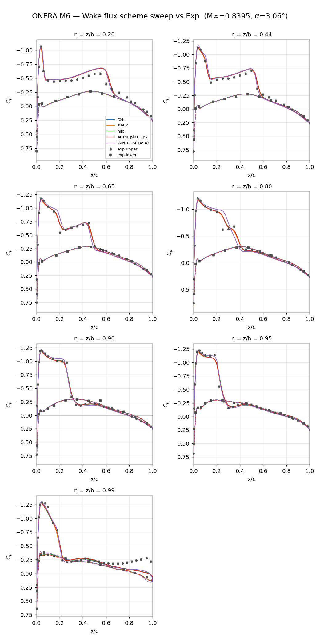
| Convective scheme | Roe (default); the example is also validated with AUSM+up2, HLLC, and SLAU2 — see Figure 2.4 |
| Results to check | Residuals, force coefficients, Mach, pressure, Cp, Cf, and y+ output |
Why a wall function here. This case uses a wall function rather than a fully wall-resolved mesh (y+ ≈ 1). Wall functions let a coarser near-wall mesh reproduce the boundary-layer velocity profile at a fraction of the cell count and run time, which keeps this quickstart fast to reproduce. For cases that need wall-resolved accuracy (separation-sensitive flows, detailed skin-friction studies), see Recommended settings and troubleshooting.
2.2 1. Copy the example to a working directory
Copy the complete examples/onera-m6-wing directory from the distribution to a working location to avoid filling the installation directory with output files. Keep JSONC files, the SU2 mesh, and any inheritance files together.
my-wake-work/
└─ onera-m6-wing/
   ├─ case.jsonc
   ├─ m6wing.su2
   └─ (required auxiliary JSONC files)
2.3 2. Run the case
Run the 3D solver from the example directory.
# Linux
/path/to/wake/bin/wake_3d_mixed case.jsonc

# Windows PowerShell
& "C:\Program Files\Wake CFD\bin\wake_3d_mixed.exe" case.jsoncThis example is a 3D case. Always use wake_3d_mixed.
2.4 3. Check the run
Review residuals and the wing-force monitor in the console.
- The calculation starts without input or mesh errors.
- Residuals decrease over iterations.
- Force coefficients stabilize toward the end of the run.
Use the history CSV to plot residuals and force coefficients. The filename is defined in the monitoring block of case.jsonc.
2.5 4. View the results
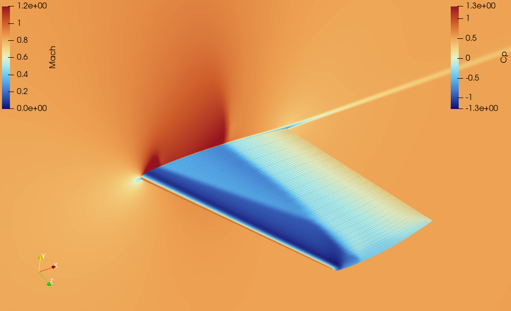
When the calculation finishes, open the volume or wing-surface results in ParaView.
- Select
MachorPressureas the color variable. - Set the view to show the wing upper surface.
- Inspect abrupt changes in Mach and pressure around the shock wave — you should see the lambda-shaped shock pattern in Figure 2.1.
- Select
Cpin the surface results to view the pressure distribution along spanwise sections. - Select
Cfandy+to check the wall-function boundary layer (Figure 2.2, Figure 2.3).y+should sit close to the target value (~30) across most of the wing, dipping locally only near the shock foot.
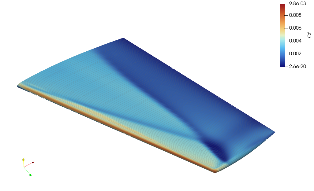
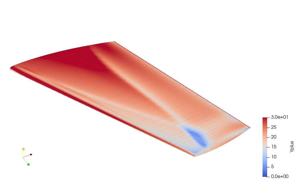
The conditions and result-review workflow for this example are based on NASA GRC ONERA M6 analysis assets. For output and monitor details, see File output and Monitoring.
Verification criterion
The installation check is complete when the solver finishes without an execution error and the Mach, pressure, or Cp field shows a flow pattern similar to the reference images above. This first run verifies that the packaged solver and example execute correctly.
For a quantitative check, Figure 2.4 compares sectional Cp from four convective schemes (Roe, AUSM+up2, HLLC, SLAU2) against the NASA GRC WIND-US published CFD solution and the original wind-tunnel experiment, at seven spanwise stations. The four schemes agree with each other and with both references across the span.