24 Monitoring

history CSV, console, residual, named monitors

24.1 What this setting is

Monitoring is the instrumentation that lets you judge, while the run is still going, whether it’s actually converging. Don’t rely on the residual alone — record whatever physical quantity actually matters for the problem alongside it: lift/drag, mass flow, a probe value. For steady analyses, judge convergence by that quantity settling, not just the residual. For unsteady analyses, judge it by the period, mean, and amplitude of that quantity settling into a repeatable pattern.

24.2 GUI configuration

Field	Description
Console	How often to print progress.
Residual	Whether to record the equation-residual CSV, and how often.
History file	A CSV file recording quantities of interest.
Monitor	Force coefficients, mass flow, probes, and other quantities to track.

monitoring records solver state and quantities of interest to CSV and the console at each iteration.

{
  "monitoring": {
    "history_files": [{
      "id": "main",
      "file_name": "history",
      "frequency": 1,
      "enabled": true
    }],
    "console": { "frequency": 10, "residual_basis": "scaled" },
    "solver_state": { "frequency": 1 }
  }
}

24.3 history_files

You can define several CSV streams. A monitor’s history_file refers to one by its id.

24.3.1 Choosing `frequency` for post-processing (e.g. FFT)

If a history CSV feeds a frequency-domain analysis later — extracting a vortex-shedding frequency from a force-coefficient trace, for example — the effective sampling rate is 1 / (frequency · Δt). For a valid FFT read this needs to clear the Nyquist limit (at least twice the frequency you’re trying to resolve) with real margin, not just barely. In practice this is rarely a real constraint: at a physical timestep chosen to already resolve the phenomenon well (say, several hundred steps per expected period, as is typical for an implicit BDF run), recording every iteration (frequency: 1) oversamples by two to three orders of magnitude relative to Nyquist — harmless for FFT quality, and cheap in disk terms for a scalar CSV row. Recording less often only matters if the file size itself becomes a problem (a very long explicit run with a tiny, CFL-driven Δt can otherwise produce a multi-hundred-thousand-row CSV) — in that case, dropping frequency to, say, every 100 or 1000 iterations still leaves enormous Nyquist margin for anything in the audible-vibration-to-shedding frequency range.

24.4 console

Prints iteration status to the console every frequency iterations.

{
  "monitoring": {
    "console": {
      "frequency": 10,
      "residual_basis": "scaled"
    }
  }
}

residual_basis selects which basis the console residual column is displayed on.

Value	Display
`scaled` (default)	`R / R₀` — orders of magnitude dropped from the start. Mean-flow `R₀` is the max over the first 5 iterations; turbulence equations use `‖a_p·φ_p‖`.
`absolute`	Raw `log10(L2 RMS)`.

scaled uses the same basis as the run_control.convergence.residual_reduction criterion. Which mode is active is announced once in the console right after the solver starts.

This key only affects the console column. The CSV always writes both bases to separate files — solver_residual.csv is absolute, and solver_residual_reduction.csv is scaled.

24.5 print_inner_iter

A sibling of console and solver_state, not nested under either — it applies symmetrically to both. In dual-time (bdf1/bdf2) unsteady analyses, setting it true prints/records the inner (pseudo-time) row instead of the outer physical-step row, for both the console and the solver_state CSVs.

{ "monitoring": { "print_inner_iter": false } }

24.6 solver_state

A separate stream that records solver_residual.csv (and its companions, solver_residual_reduction.csv and the time-integration log). The default frequency is 1 for DBNS/PBNS and 20 for FR; an explicit value overrides that. 0 records only the final iteration.

{
  "monitoring": {
    "solver_state": {
      "frequency": 1,
      "console_fields": ["Flow_Res", "Flow_Rho", "CFL_Max", "Wall_Time"]
    }
  }
}

There’s no enabled flag here — this stream is the run’s convergence record, not a display you toggle off; to write less of it, raise frequency (even 0, final-iteration-only, still gives you the minimum record).

console_fields picks which residual/CFL columns appear on the console, replacing the default expansion (one column per residual variable, plus CFL). It takes solver-exposed scalar names (Flow_Res, CFL_Max, Wall_Time, and so on) — not the names of your own monitors[] blocks. A monitor’s console column is controlled by that monitor’s own console: true, independently of this key.

24.7 monitors

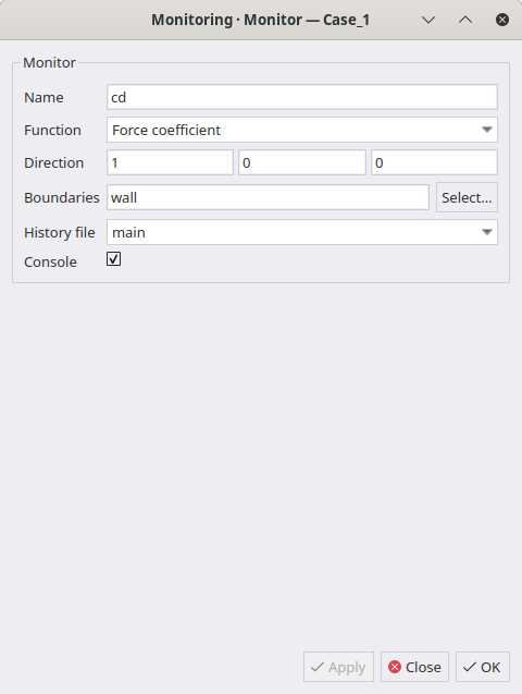
Wake CFD Desktop Monitor dialog defining a drag coefficient monitor on the wall boundary and routing it to history and console output — Figure 24.1: A force-coefficient monitor projected in the x direction, integrated over the named wall boundary, routed to the main history file, and shown on the console.

The GUI changes the available rows when Function changes. The selected values are written to one entry in monitoring.monitors; the JSONC form below shows the same contract and also documents functions not visible in this particular capture.

A monitor is defined by three axes — where (target), how (function), and, for functions that need it, what (variable). Every function’s primary output is a single scalar; the block’s name is both the CSV column name and the console column name (when console: true).

{
  "monitoring": {
    "monitors": [
      {
        "name": "CFy",
        "target": { "boundaries": ["AIRFOIL"] },
        "function": "force_coefficient",
        "direction": [0.0, 1.0, 0.0],
        "history_file": "main",
        "console": true
      },
      {
        "name": "CFx",
        "target": { "boundaries": ["AIRFOIL"] },
        "function": "force_coefficient",
        "direction": [1.0, 0.0, 0.0],
        "history_file": "main",
        "console": true
      },
      {
        "name": "CMz",
        "target": { "boundaries": ["AIRFOIL"] },
        "function": "moment_coefficient",
        "axis": [0.0, 0.0, 1.0],
        "origin": [0.25, 0.0, 0.0],
        "history_file": "main",
        "console": true
      },
      {
        "name": "wake_pressure",
        "target": { "point": [2.0, 0.5, 0.0] },
        "function": "probe",
        "variable": "Pressure",
        "history_file": "main"
      },
      {
        "name": "lift_to_drag",
        "function": "expression",
        "expression": "CFy / CFx",
        "history_file": "main"
      }
    ]
  }
}

24.7.1 `target`

Form	Meaning
`{ "boundaries": [...] }`	A surface function integrated/evaluated over one or more named boundaries.
`{ "point": [x, y, z] }`	A probe: sample the flow field at a single point.
(omitted)	Only valid for `function: "expression"`, which references other monitors instead of the flow field directly.

24.7.2 `function`

Function	What it computes	Needs `variable`?
`force`, `force_coefficient`	`∮(p − p∞)n̂ dA + ∮τ̿·n̂ dA`, projected onto `direction` (`force_coefficient` also divides by `q∞·S_ref`)	No
`moment`, `moment_coefficient`	`∮r⃗ × (stress) dA`, projected onto `axis` about `origin` (default: `reference.origin_moment`)	No
`area`	`∮dA`	No
`mass_flow`	`∮ρV·n̂ dA`	No
`momentum_flux`	`∮ρ(V·n̂)² dA`	No
`integral`	`∮φ dA`	Yes
`area_average`	`∮φ dA ÷ A`	Yes
`flow_rate`	`∮(ρV·n̂)φ dA` — signed physical flux of `φ`	Yes
`mass_average`	`∮φ\\|ρV·n̂\\| dA ÷ ∮\\|ρV·n̂\\| dA` (backflow-safe)	Yes
`probe`	Point sample of `φ`	Yes
`expression`	Evaluates `expression` against other monitors’ values (no `target`)	No

variable takes a FlowVariable name and is only accepted by the five functions above that use it — supplying it elsewhere (or omitting it where required) is rejected at validation time.

Tip

Force and moment monitors on the same target share a single GPU reduction — defining all six body-axis components (CFx/CFy/CFz/CMx/CMy/CMz) on the same boundary set costs one surface integral pass, not six. There is no composite “all six at once” monitor anymore; write one block per component and let the shared-target reduction absorb the cost.

direction (force) and axis (moment) don’t have to be a coordinate axis — the old body-axis CFx/CFy is just the special case direction = [1,0,0] / [0,1,0]. For wind-axis CL/CD at angle of attack α, write direction: [-sin α, cos α, 0] (lift) / [cos α, sin α, 0] (drag) explicitly — the solver normalizes whatever vector you give it.

If a viscous run’s target includes a no-slip wall, force/moment monitors automatically get two extra CSV columns, <name>.pressure and <name>.friction, decomposing the total (CFy ≈ CFy.pressure + CFy.friction). An inviscid run only ever has the one total column.

Warning

A scalar function (area, integral, area_average, …) applied to several boundaries at once does not sum across them — it produces one column per boundary, named <name>.<boundary>. There is no plain <name> column to put on the console for a multi-boundary scalar monitor; reference the individual <name>.<boundary> columns instead (including in run_control.convergence.monitor.fields).

24.8 Time-averaging a monitor

A monitor doesn’t take the time_average.fields used by output blocks — averaging applies to the monitor’s entire scalar output instead.

{
  "monitoring": {
    "monitors": [{
      "name": "cd_mean",
      "target": { "boundaries": ["AIRFOIL"] },
      "function": "force_coefficient",
      "direction": [1.0, 0.0, 0.0],
      "history_file": "main",
      "console": true,
      "time_average": {
        "enabled": true,
        "start_iter": 500,
        "rms": true
      }
    }]
  }
}

The old flat statistics_* keys are no longer used.

24.9 Setting this from the CLI

{
  "monitoring": {
    "console": { "frequency": 10 },
    "solver_state": { "frequency": 1 },
    "history_files": [{
      "id": "main",
      "file_name": "history",
      "frequency": 1,
      "enabled": true
    }]
  }
}